
Random Quote Board
Gnu Radio & Frequency Demodulation - Why Not Some More?
It turns out that the rabbit hole of "How many different ways can you make a frequency demodulator?" digitally is far deeper than I imagined. It's my fault. I asked a former co-worker, and also one of the most brilliant engineers alive, if he had any ideas on digital frequency demodulation.
I was not disappointed.
The Zero-Crossing Pulse Count Discriminator
In my last post, I had a heading for a "Zero-Crossing Discriminator" and stated:
Yet another of the techniques that I've not yet figured out how to mimick in GRC. Nuf said.
Guess what? Thanks to my former co-worker, I figured it out.
He briefly discussed a pulse counting discriminator. He then pointed me to a Youtube video of a pulse count FM discriminator. This discriminator works by creating an impulse at the zero-crossings of the FM signal. FM, as the name states, varies the frequency of the carrier. The higher the amplitude of the baseband signal, the higher the frequency of the carrier. The same is true if the amplitude of the baseband signal is lower. The lower the amplitude, the lower the frequency.
A basic tenet of signals is that frequency and period are inversely related. If the frequency of the carrier sine wave is increasing, then the period is decreasing. If the period decreases, this means that more zero-crossings occur within a certain amount of time. The lower the frequency, the fewer the number of zero-crossings.
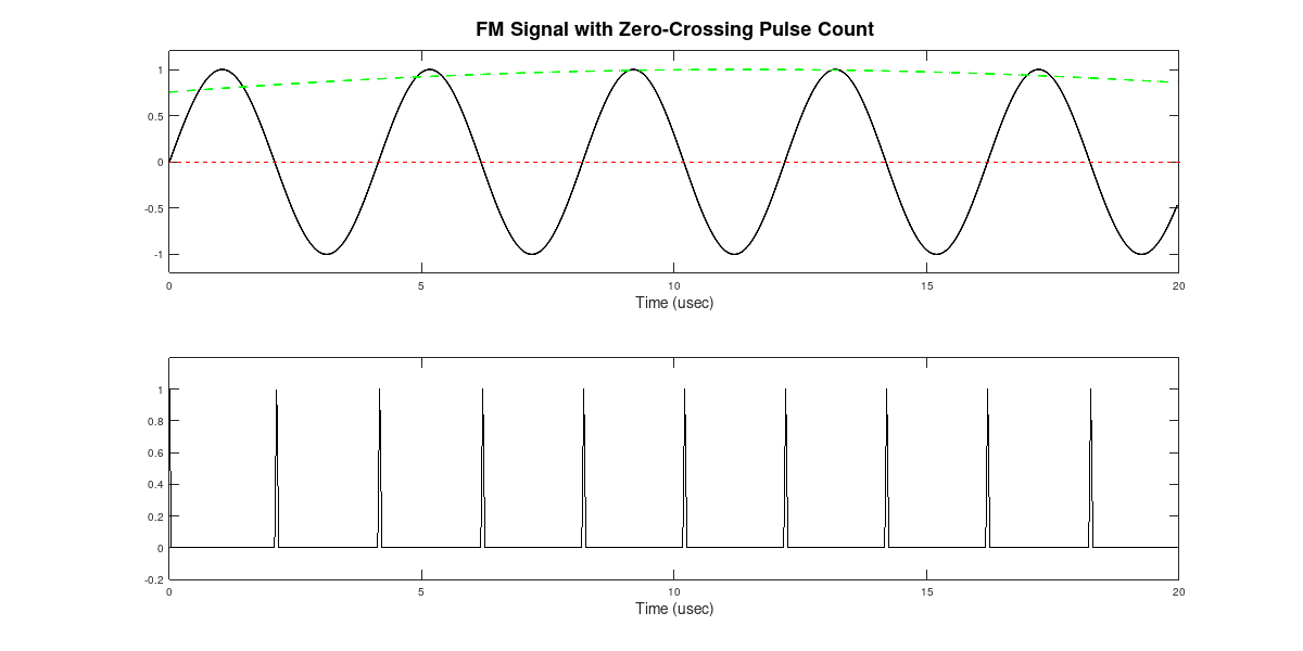
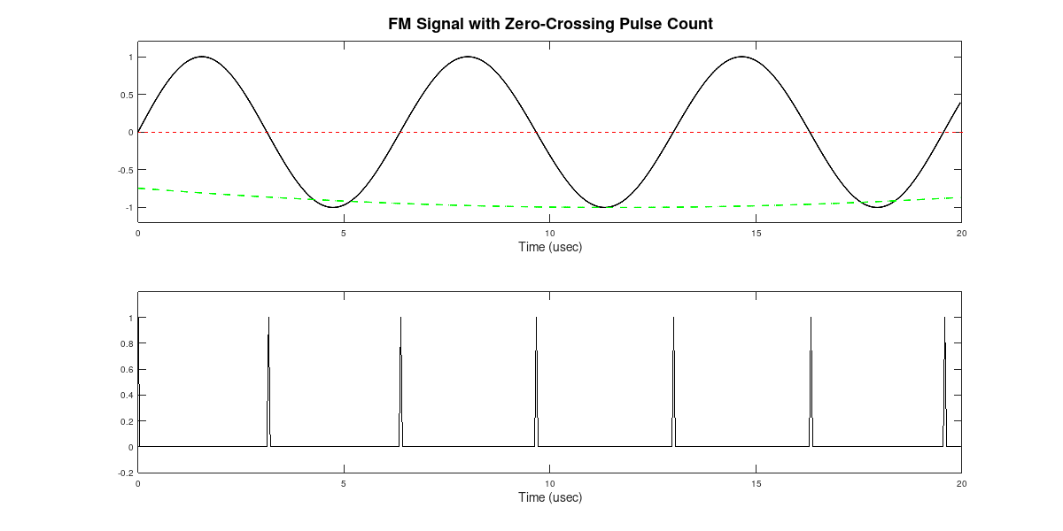
A lowpass filter will act as a "counter". It will average the energy of the pulsed signal. With more pulses, the average will be higher; it will be lower with fewer pulses.
The problem here was that I cannot program computers. I can do some basic HTML and CSS, as this website attests. (I program this entire site using Text Editor (in Linux) or Notepad++ (in Windows).) I can also do some basic Gnu Octave / Matlab. Beyond that? Yeah, I can do some "Hello, World!" C and C++ basics. But that's it. This meant that, unless I could figure out how to use Gnu Radio Companion's already-available blocks, I couldn't make the pulse counting circuit digitally.
Here's what I figured out.
- The pulse counting circuit only works on real, not complex, samples. I may be wrong. I could not figure out how to make the circuit work on complex samples. But I did figure out how to make it work on real signals.
- Zero-crossings occur where one consecutive sample is positive and the other is negative. The probability that a particular sample will land exactly on zero is extremely small. This means that consecutive samples will straddle the zero line. Starting with the real signal, it's possible to create a one-sample delayed version of the real signal, then multiply that stream with the stream of undelayed samples. At a non-zero crossing, both samples will be either both positive or both negative. By multiplying the undelayed and delayed streams together, the product will be positive at a non-zero-crossing. The product will only be negative at a zero-crossing.
- The negative samples (described above) and the GRC "Rail" block can create impulses. As described above, GRC can be used to create a set of samples that are only negative at zero-crossings of a waveform. The problem is that these samples are intermingled with all of the positive samples from the non-zero-crossing points. How can we separate them? Using GRC's "Rail" block. That block allows for samples to be altered based on their amplitude. By setting the values such that all positive samples get set to zero, then that eliminates the non-zero-crossing samples. The ones that are left will be the impulses of the zero-crossings.
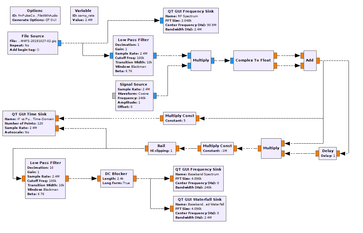
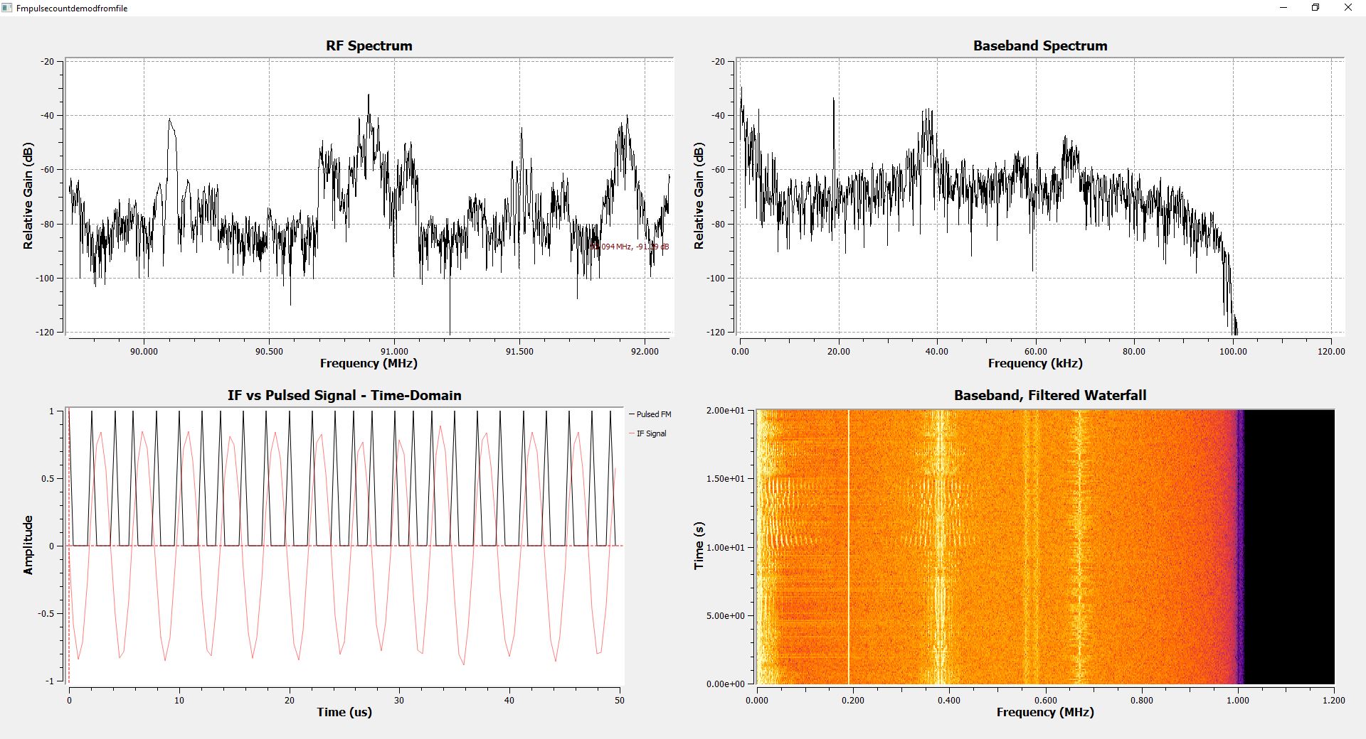
Much to my surprise, this GRC graph actually works. One thing I noticed was that there was a distinctive crackling in the background. Here's what I think is happening. The first lowpass filter works on a set number of samples at a time. GRC calculates that number of taps (samples) using the "harris approximation". The calculation shows that, with the given parameters (Blackman window, 2.4 MHz sample rate, 10 kHz transition width), the lowpass filter will operate on 808 samples. With a IF of 240 kHz, this equates to roughly 81 cycles of the FM signal with no modulation. FM broadcast uses a 75 kHz deviation, so the frequency limits will be 240 kHz +/- 75 kHz, or 165 - 315 kHz. At the lowest frequency limit, the IF will have 55 1/2 cycles over the course of the filtering, while the high frequency limit will have 106 cycles. The graph generates two impulses per cycle (one for the positive going and one for the negative going). This means that GRC will generate between 111 - 212 impulses, depending on the frequency of the FM carrier at each point. The number of impulses counted will be an integer number. The input to the lowpass filter will be a sum of integers somewhere between 111 and 212. If my hypothesis is correct, this means that the dynamic range is limited to roughly 212 - 111 = 101, or roughly 40 dB. This is less than a vinyl LP. Hence, the crackling in the background is probably quantization error of the integer number of impulses.
| This is the demodulated audio from an FM broadcast station using the pulse counting GRC graph above. |
The Delay Line Discriminator
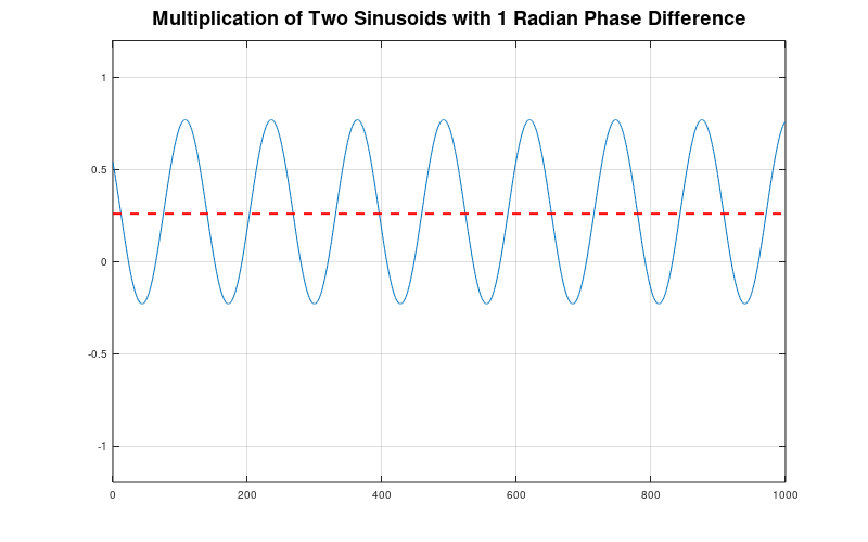
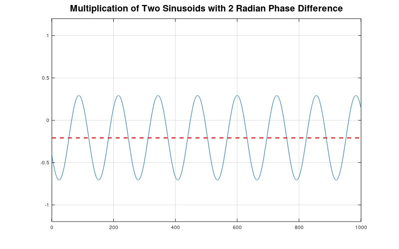
Here's the thing about multiplying two sinusoids that are the same frequency. If they have a phase difference of π/2, you wind up with a sinusoid that is twice the frequency of the two, original sinusoids. (Note: It's actually the sum of the frequencies of the two, original sinusoids.)
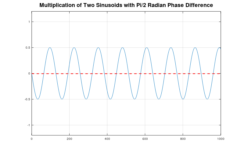
But what if the phase difference is either more or less than π/2? The product will still have a frequency of (roughly) twice the original sinusoid frequency. But the DC offset will vary depending on whether the phase difference is more or less than π/2. With a phase difference less than π/2, the DC offset will be greater than zero. Conversely, a phase difference of greater than π/2 will lead to a DC offset less than zero.
This leads to the delay line discriminator. We can use a digital delay to set the delay to the equivalent of 1/4 of a cycle. This is a phase delay of π/2 radians. What happens if we increase the frequency of the signal? The digital delay remains the same (X number of samples). But the signal will shift a greater number of radians between samples because it is a higher frequency. The converse is true if the frequency of the signal is lower. With a lower frequency, the phase difference will be less than π/2 radians. Thus, with a FM signal, as the frequency varies above and below the IF center frequency, multiplying the signal with a 1/4 cycle delayed version of itself will create two signals. The first signal will be a varying-frequency sinuosoid centered on twice the IF. The second will be a varying-amplitude DC offset. A lowpass filter will remove the 2x-IF signal. This leaves the varying-amplitude DC offset based on the varying frequency.
Here's an interesting tidbit. The circuit will still work even if the delay is not equivalent to a π/2. The difference is that, with a delay of precisely a π/2, when the signal is at its center frequency, the average will be zero. This means the output, demodulated signal will have no DC offset that requires a DC blocker circuit. Don't take my word for it. Try the circuit below yourself and set the delay to 2 or 4 samples. It will still work. It's just that there will be a greater DC offset for the DC blocker to, uh, block.
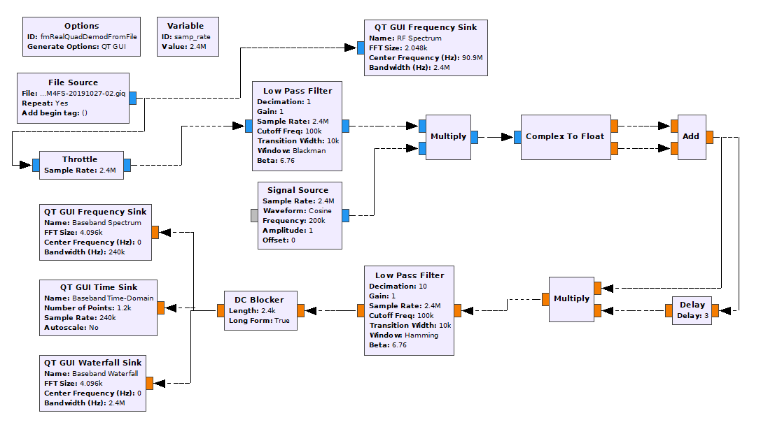
| This is the demodulated audio from an FM broadcast station using the delay line discriminator GRC graph above. |
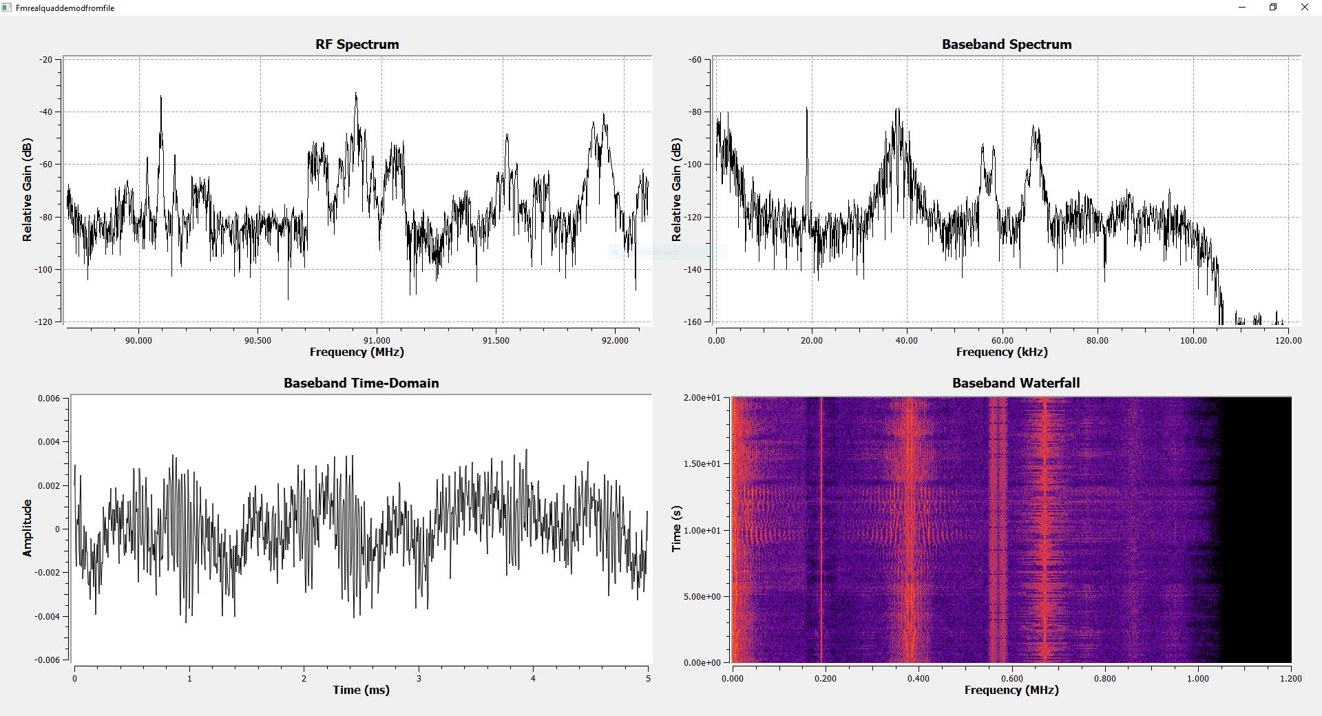
The Baseband Delay Demodulator
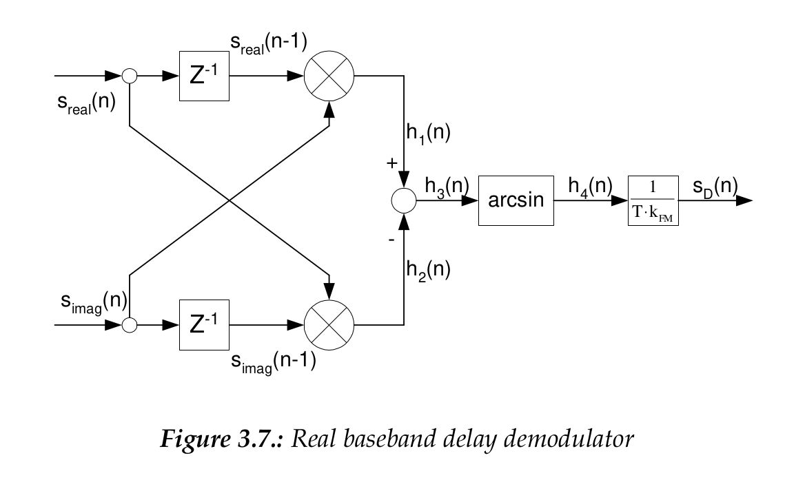
UPDATE: Yeah. There's another one. I found it while reading through "Implementation of FM Demodulator Algorithms on a High Performance Digital Signal Processor" by Franz Schnyder and Christoph Haller from Nanyang Technological University in Singapore. Specifically, they derive a "baseband delay demodulator" that is, essentially, another version of the polar discriminator (as shown in Figure 3.6). The difference is in how it is implemented. By using the components of the complex baseband signal separately, their flowgraph uses the arcsin rather than the arctangent.
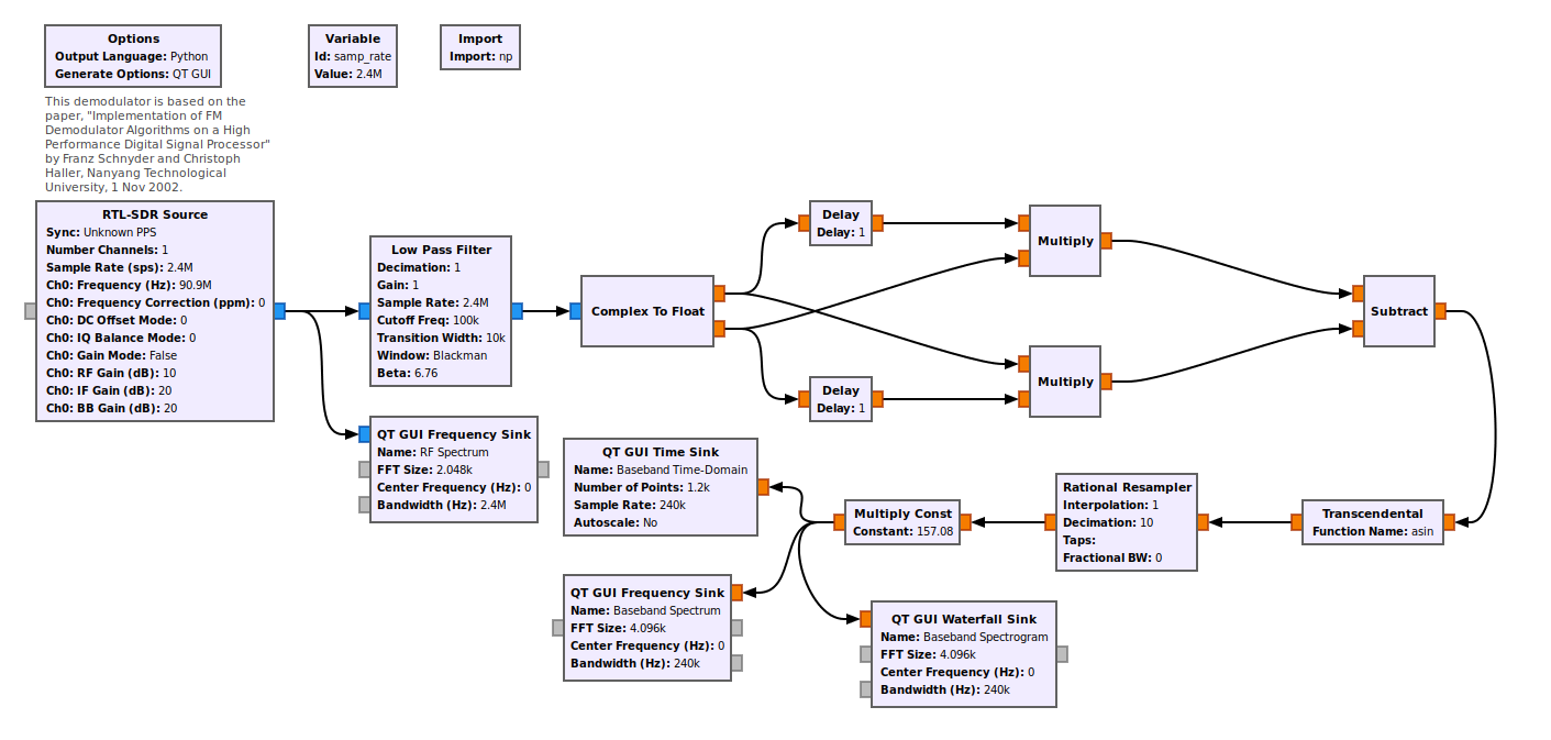
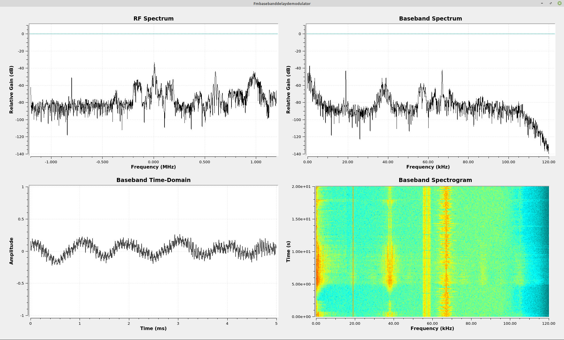
It works just fine. Despite the fact that these different discriminators were designed for narrowband FM signals, this one (at least) seems to work just fine on wideband FM signals. I also decided to simply add this one, last (probably?) FM discriminator on this post, rather than make a new post for it. Call me lazy.
Conclusions
As I was working on this, it dawned on me that the delay line discriminator is (probably) the closest I can come to the Foster-Seely discriminator. The Foster-Seely discriminator uses a combination of voltage and current variations in a transformer to demodulate FM signals. The difference is that the Foster-Seely uses the current phase changes, while the delay line uses the voltage phase changes.
With this, the pulse count discriminator, and the baseband delay demodulator, I think I can finally put a rest to all of the possible digital FM demodulators.