
Random Quote Board
Gnu Radio Companion Frequency Demodulators
I'd like to acknowledge and thank the wonderful author Richard G. Lyons and his book "Understanding Digital Signal Processing" for much of the knowledge that made this post (and several that will follow) possible.
I've been playing around quite a bit with various software defined radios (SDRs) and Gnu Radio Companion. I initially found a lot of different websites with tutorials. How to create a basic graph. How to connect the blocks. Like probably many of you out there, my first working graph was a FM receiver. After I got my first one working, I went a little... deep... down the rabbit hole trying to understand how it worked. The following is the result of that rabbit hole mapping.
FM Demod and the "WBFM Receive" Block
The first FM receiver I created used the "WBFM Receive" block, as shown below.
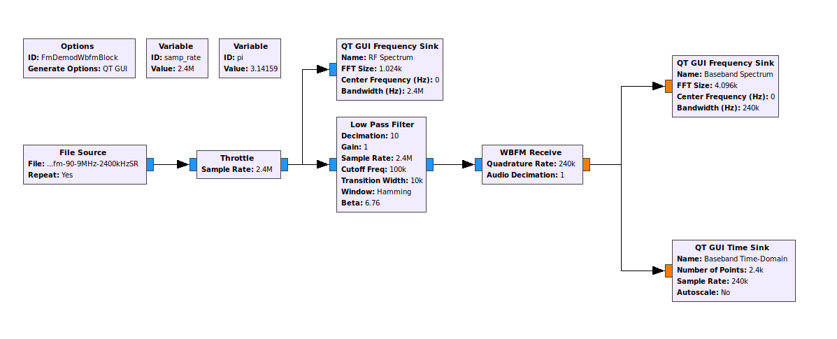
I'm the type of person who really wants to understand what's going on. While I was playing around, I discovered that the "WBFM Receive" block used another block called "quadrature demod". When I looked into it, I discovered that the "quadrature demod" was a specific form of frequency demodulator. The "WBFM Receive" block actually ties two blocks together. The first is the "Quadrature Demod", which performs the frequency demodulation. The second is a decimator, which reduces the bit rate. While it is not part of the parameters of the "WBFM Receive" block, there also appears to be a lowpass filter. I'll explain why I believe that shortly.
FM Receiver Using the Quadrature Demod Block
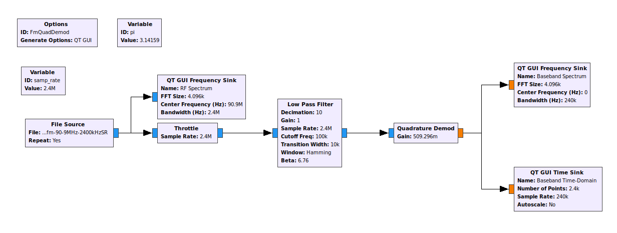
I decided to create a slighly different graph, this time using the "Quadrature Demod" block in place of the "WBFM Receive" block. It has one adjustable parameter, called the "Sensitivity". The "sensitivity" of this block is nothing more than a scaling factor. It's initially based on two things, the sample rate and the number of radians in a circle (2π). When you initially open the sensitivity value, it has three parameters by default. These are the sample rate, the value "2π", and an FSK deviation. The FSK deviation is for something else, and despite the fact that it is included by default, it's not needed.
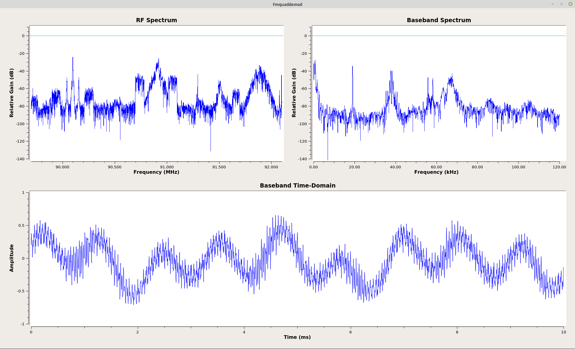
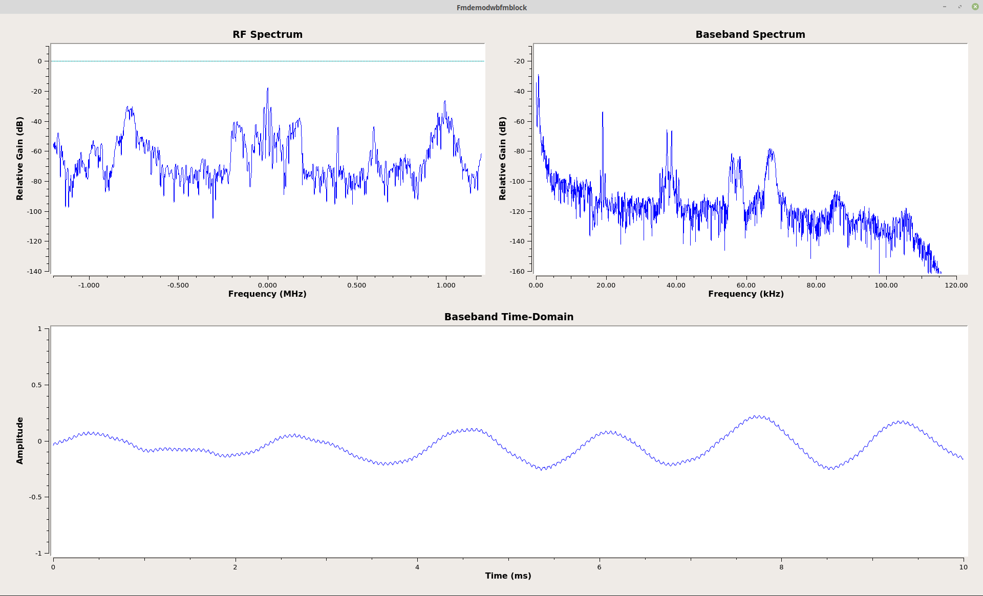
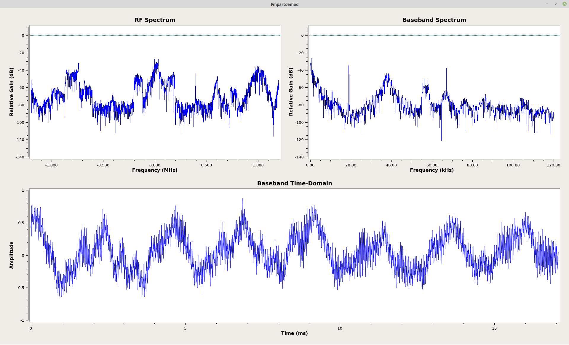
You may be wondering, "Where's the audio output?" I didn't need an audio output to know that the signal was demodulating properly. The appearance of the baseband spectrum tells me everything I need to know. Here's what the spectrum tells me.

This is how the baseband spectrum of a FM broadcast signal should appear. Some signals do not have the stereo signal (such as talk radio shows), many do not have the SCA, and some do not have the RBDS. But this one does, and the spectrum is precisely as it should be.
So how is the "Quadrature Demod" block demodulating the signal?
This still does not explain what is actually going on in the "Quadrature Demod" block. To see that, you have to look at the documentation of the block itself. It says:
This can be used to demod FM, FSK, GMSK, etc. The input is complex baseband, output is the signal frequency in relation to the sample rated, multiplied with the gain.
Mathematically, this block calculates the product of the one-sample delayed input and the conjugate undelayed signal, and then calculates the argument of the resulting complex number:
y[n] = \mathrm{arg}\left(x[n] \, \bar x [n-1]\right).
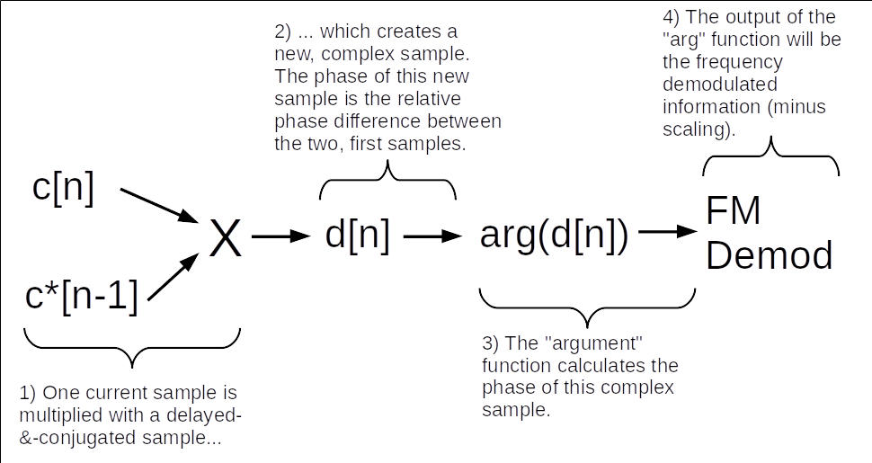
Yes, that is some interesting mathematical guacamole right there. Here's what the text says:
\( \Large y[n] = \arg (c^* [n] \times c[n-1] ) \)
Where:
- y[n] = FM demodulated output
- c*[n] = complex conjugate sample (take a complex sample and invert the sign of the imaginary part)
- c[n-1] = complex sample delayed by one sample period
- arg = argument, which is a special form of calculating the arctangent.
UPDATE Feb 2021: When I originally wrote this post, the documentation for the "Quadrature Demod" block said that the non-delayed sample was conjugated. I originally thought the same thing, and my original post said as much. The equation (written in a a set of Tex commands) for the "Quadrature Demod" block says:
\( \Huge y[n] = \mathrm{arg}\left(x[n] \, \bar x [n-1]\right) \)
This equation is correct. The documentation, and this post, have since been corrected.
This is a polar discriminator. A polar discriminator is a way to calculate the relative phase difference between two complex samples. It multiplies two complex samples, where one sample is conjugated (the sign of its imaginary component is inverted) and the other sample is delayed one sample period. The result of the multiplication is a third complex sample. The phase of that new complex sample is the phase difference between the two, original samples. The last step is to actually calculate the phase of the complex sample. That is where the "argument" function comes into play. The "argument" function calculates the phase of a complex sample.
Frequency is a difference of phase over time, or Δθ / Δt. We've calculated the difference in phase (Δθ). We now need the "Δt". That is the sample period. So divide the difference in phase by the sample period. Dividing by the sample period is the same as multiplying by the sample rate. Therefore, to calculate the frequency of a signal, calculate the phase difference, then multiply by the sample rate. This is how the "Quadrature Demod" block frequency discriminates (demodulates) FM signals.
Note that the only difference between the output of the two demodulators is that the "WBFM Receive" demodulator is lowpass filtered compared to that of the "Quadrature Demod". Otherwise, they're identical. I prefer to use the "Quadrature Demod" because it gives me a better opportunity to create a stereo receiver. I'll cover that (probably) in a future post.
FM Demodulator with Polar Discriminator using Separate Blocks
Well, now that I knew how the "Quadrature Demod" block was working, I decided to see if I could make it using separate Gnu Radio Companion blocks. Based on the walk-through above, it would require a delay, a complex conjugate, a multiply, and a way to calculate the phase. Turns out that GRC has all of these components. That lead to this graph:
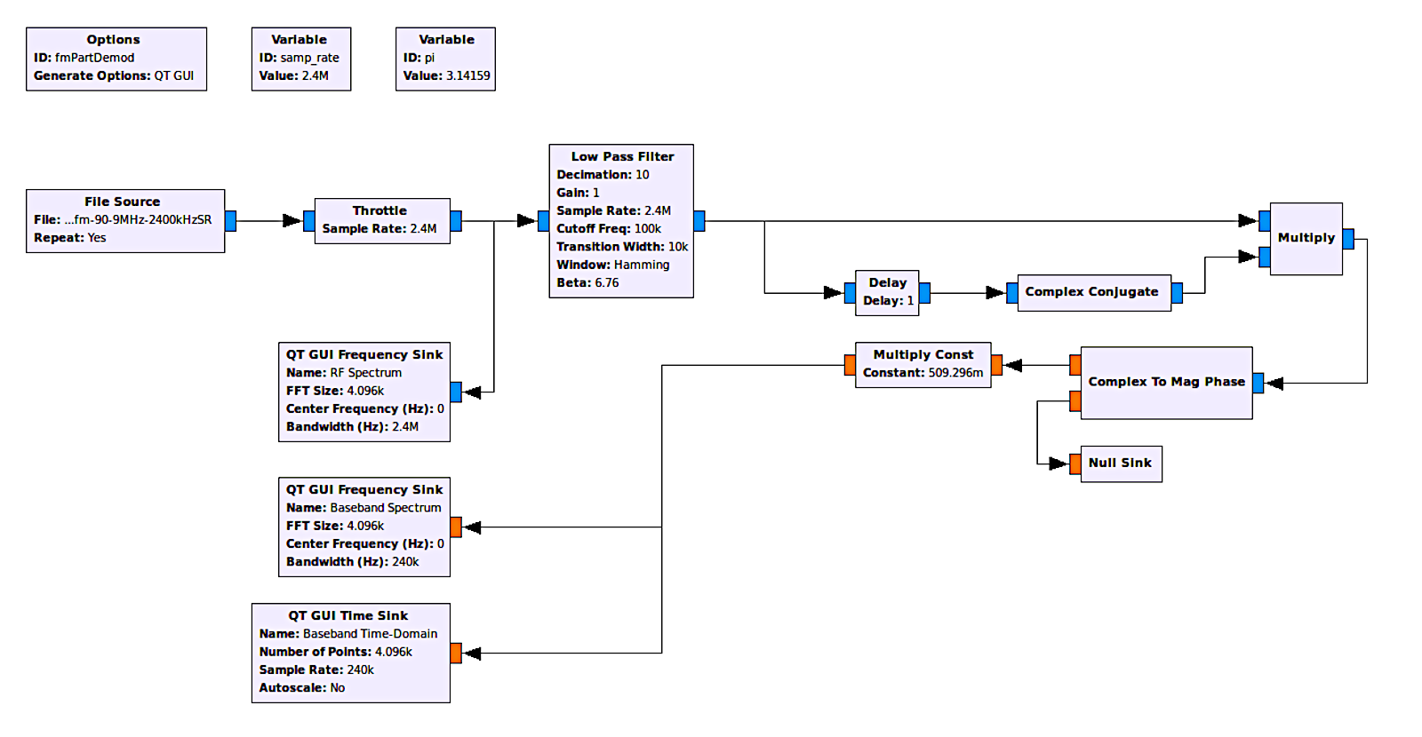
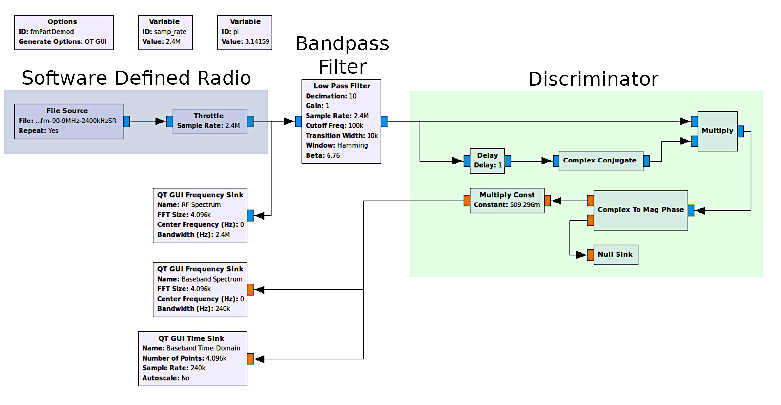
The output of this demodulator is identical to that of the "Quadrature Demod". I'm guessing that it is, in fact, identical. My guess is that it is not as efficient as having it programmed into one block, so using the "Quadrature Demod" is still the best way to go.
FM Demodulator with Polar Discriminator using Different Separate Blocks
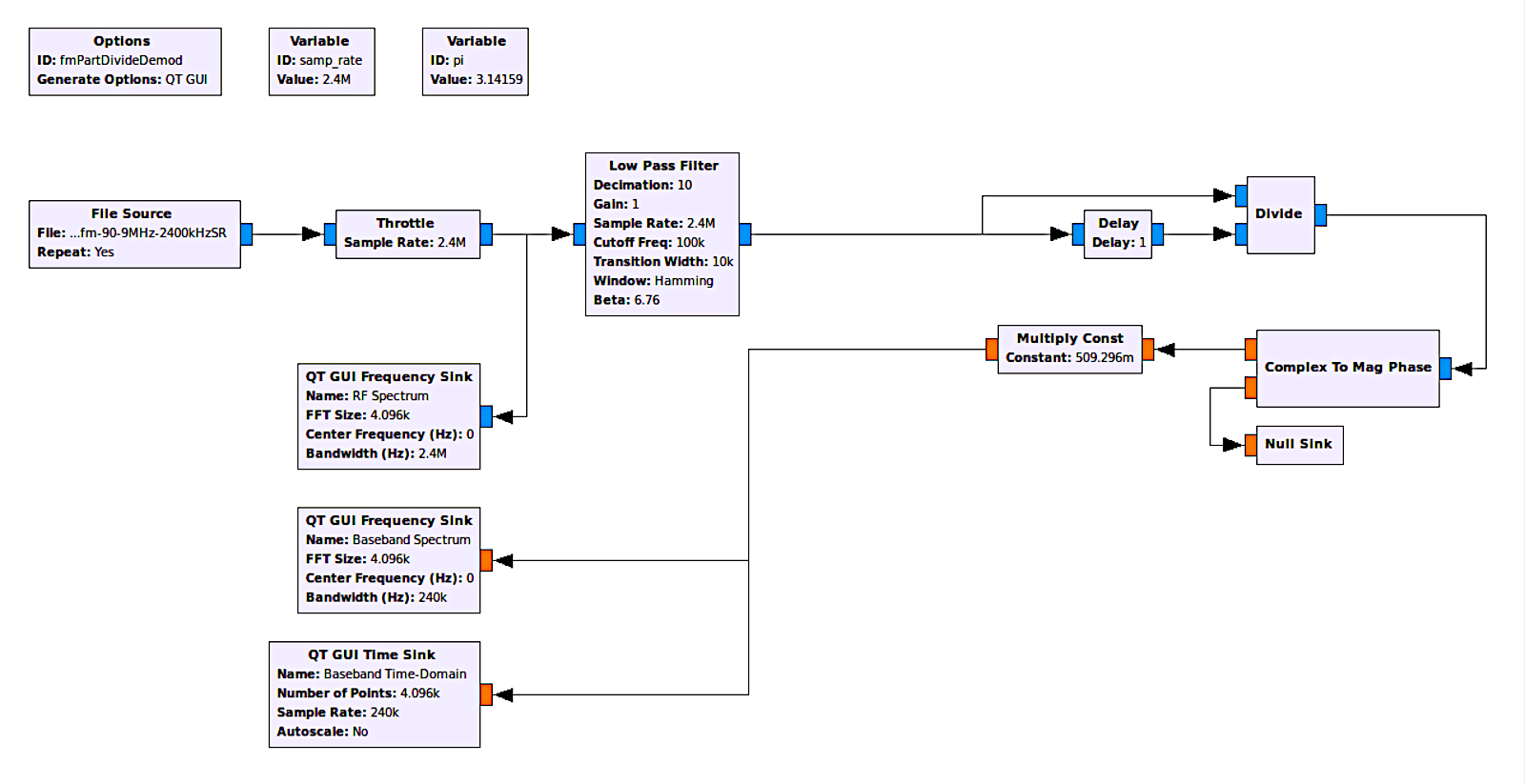
Why stop now? It turns out my research into the polar discriminator led to an epiphany. With the polar discriminator above, there's a "Complex Conjugate" block followed by a "Multiply" block. Why? Because the complex conjugate inverts the sign of the phase. This means that the multiply by a complex conjugate is similar to a divide. So why not try that? Why not remove the "Complex Conjugate" and "Multiply" blocks and just use a "Divide" block instead? Here's how that looked:
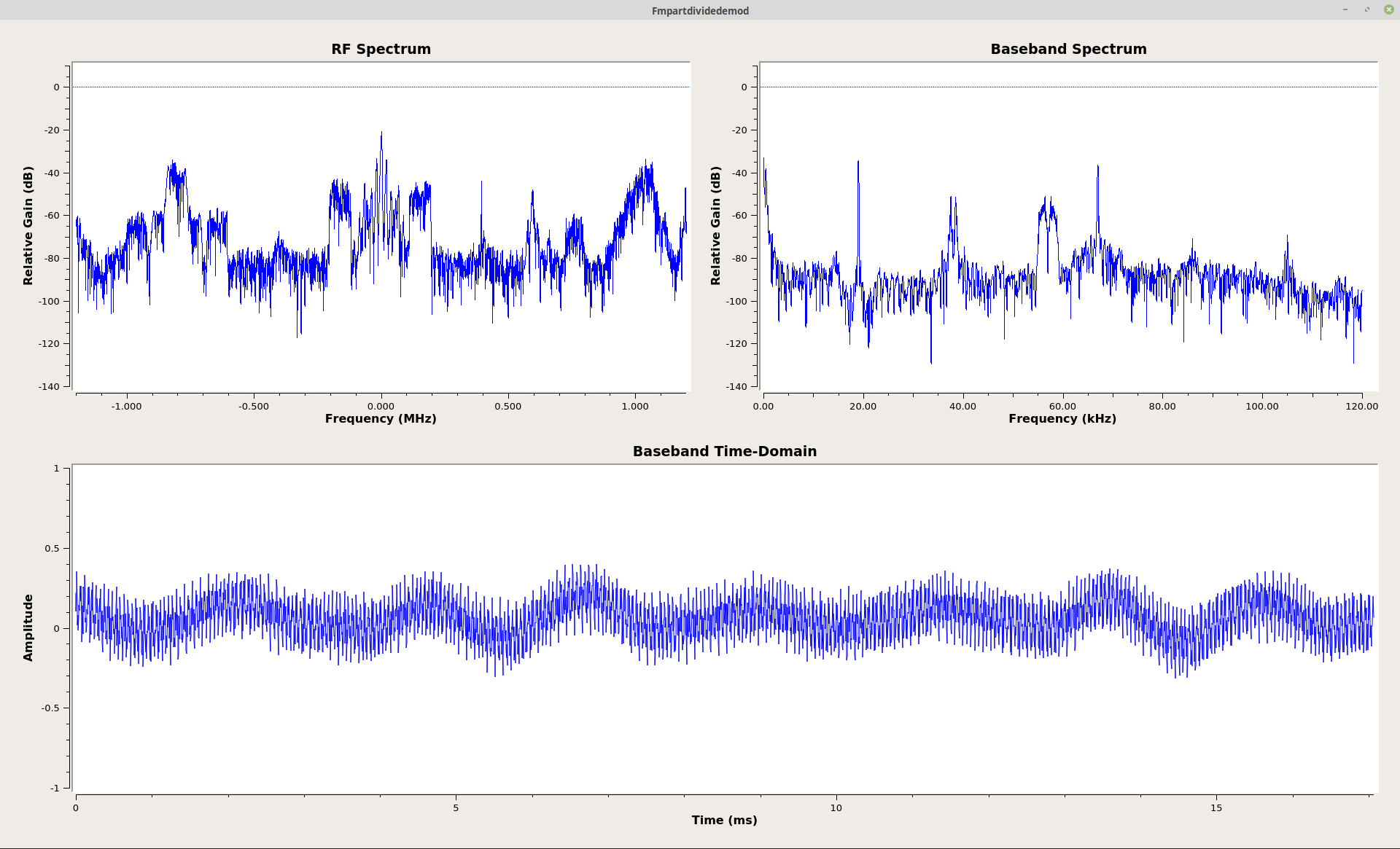
The output of this demodulator appears identical to that of the graphs using the "Quadrature Demod" and the separate parts including the "Complex Conjugate" and "Multiply" blocks. It appears that my epiphany was a correct one.
It's the little things.
Frequency Demodulator using Basic Phase Difference
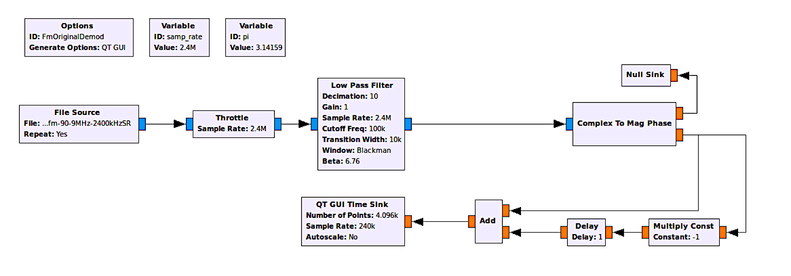
Okay, I've shown several, viable options for creating a frequency discriminator using (slightly) different methods and components. All of the above use the polar discriminator method. However, when I first started looking at frequency demodulators in the digital domain, I used a much more complicated method. As I said above, frequency is a change of phase over time. I've been studying digital signal processing for some time. Several years ago, I created my first digital demodulator in Mathcad. I did this by calculating the phase of each sample individually, then subtracting one phase from the previous one. I no longer use Mathcad (I'm more of a Gnu Octave user now), but I decided to try this technique in GRC. This lead to the following graph:
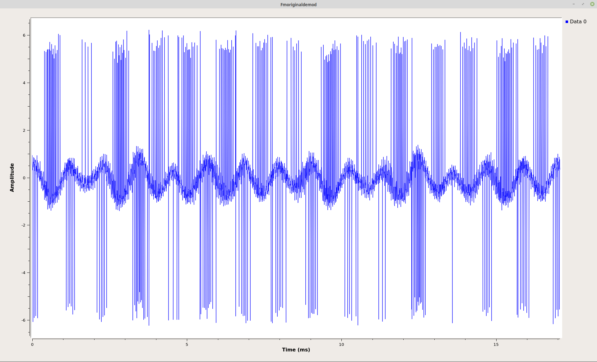
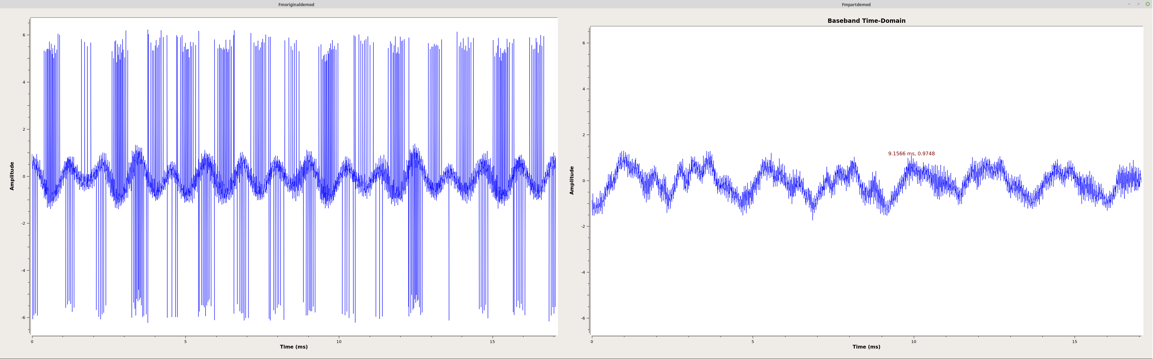
The graph above sorta / kinda works. You can see the baseband signal in the time-domain (shown above, left), especially when compared to the time-domain baseband from the "Quadrature Demod" block (above, right). But it's covered in impulsive noise. That's due to the subtraction part of one phase from another. The absolute values of the phase run between +/-π. But what if one value is, for example, near -π and the next near +π? The difference will then shoot up to somewhere near +/-2π. Those are the impulses shown above. In my original Mathcad worksheet, I used Mathcad's conditional functions (namely an "if/then" loop) to account for this. If a value had an absolute value above π, subtract that value from 2π. It worked. However, GRC does not have a conditional block I can use. This means that this is as good as it is going to get. In other words, this is not a viable option for a frequency demodulator in GRC.
Frequency Demodulator Without the Arctangent Function
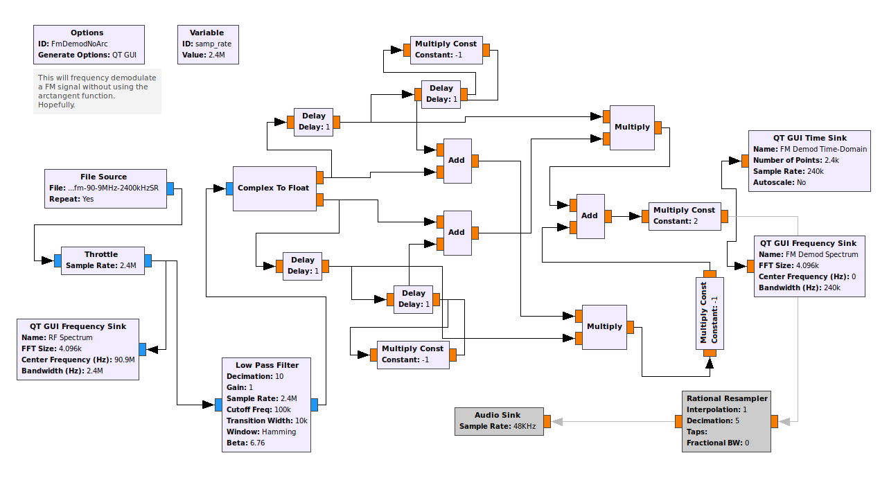
All of the frequency demodulators above require calculating the phase of a complex sample. That means using an "arctangent" function. That can be computationally expensive. In his book "Understanding Digital Signal Processing", Richard G. Lyons derives a frequency demodulator that does not use the arctangent function. As I looked at the diagram marked 13-61(b) in the book, I realized that GRC had every component necessary to make it work. That lead to the following, quite complicated graph:
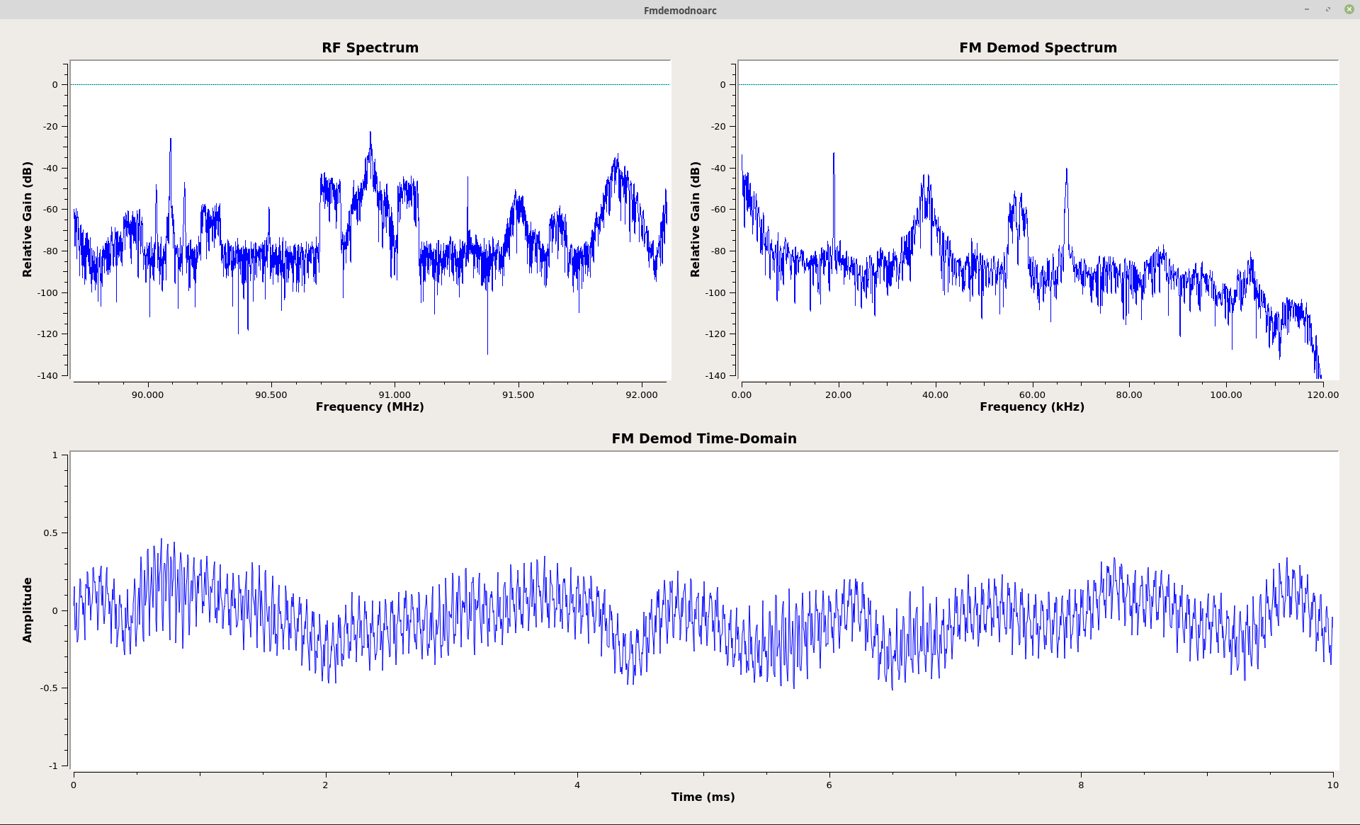
As you can see from the displays above (right), it works! You'll also note that there is an audio sink on this block. I didn't have that in the others for the simple reason I didn't need to hear the audio. Shortly after I got this working, in my excitement, I sent an e-mail to Mr. Lyons explaining how I was able to get his technique to work in Gnu Radio. A few minutes later, I received a response. He wanted to chat by phone.
That's right. The author of one of the best and most popular books on digital signal processing wanted to talk.
To me.
So we did. Those audio blocks in the graph above? Those were for him. As I was talking to him, I added those blocks, then played the audio from the graph using his technique. I wanted him to hear the result of his brilliance.
Wrap-up & Future Work
I hope you've learned something reading this. At the very least, I hope you understand how the frequency demodulator in Gnu Radio works.
As I get the time, I'm working on future posts to cover more general topics in complex sampling and digital signal processing, all using GRC. It provides a hands-on experience that is not available (or is more difficult to use) anywhere else.
To Delay-and-Conjugate, or Not?
This is a correction to the original post. This is based on a string of e-mails with Mr. Lyons. He'd sent me James Shima's thesis paper outlining the polar discriminator. It was during that exchange that we noticed that there was a difference between Shima's paper, and the description of Gnu Radio's quadrature demodulator. After a bit of research, we determined that Shima was correct. A polar discriminator using a delayed-and-conjugated sample multiplied with a current (and unchanged) sample produces the correct output. By "correct output", we mean that a higher frequency deviation of the carrier will produce a positive output, and a lower frequency deviation will produce a negative output.
Looking at it from the perspective of a polar plot, this means that a motion in the counter-clockwise (positive phase) will correspond with a higher frequency deviation; a clockwise (negative phase) will correspond with a lower frequency deviation.
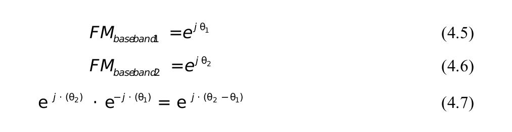
This led me to another question. Why did the polar discriminator work without a decision circuit, whereas a straightforward phase discriminator did not? What is it about multiplying the complex sample with a previous sample (that is also conjugated) that makes it work without having to worry about the "wrap around" problem? If you look at Shima's equations, multiplying the two complex samples in exponential form simply adds the phases. So, if we have a point that has a phase of, say, 5π/6 and another at -7π/8, the difference angle between them crosses the boundary between +π and -π. A straight subtraction of the phases would be 5π/6 - (-7π/8) = 41π/24. This is larger than π.
The answer is that the complex multiplication takes place using Cartesian coordinates, not exponentials. This means that we're not actually adding the phases; we're multiplying the real and imaginary components together, and the product sample will have a phase that is equivalent to the difference phase between them. And the difference phase, due to the fact that it was arrived at using Cartesian coordinates, will have a phase whose absolute value will always be less than π. Again, due to the fact that the polar discriminator uses Cartesian coordinates for calculating the phase difference, it does not require a decision circuit (if-then-else) to ensure the difference phase is always falls between -π and π.