
Random Quote Board
Understanding the hackrf_sweep Command
Overview of Sweeping Spectral Displays
Great Scott Gadgets, maker of the HackRF One and HackRF Pro, have also released a set of command line, software tools for the HackRF. One of those tools is hackrf_sweep. This command allows a person to essentially create a sweeping or swept spectrum analyzer, similar to a swept-tuned spectrum analyzer. NOTE: I use swept-tuned spectrum analyzer for older, analog-based spectral displays.
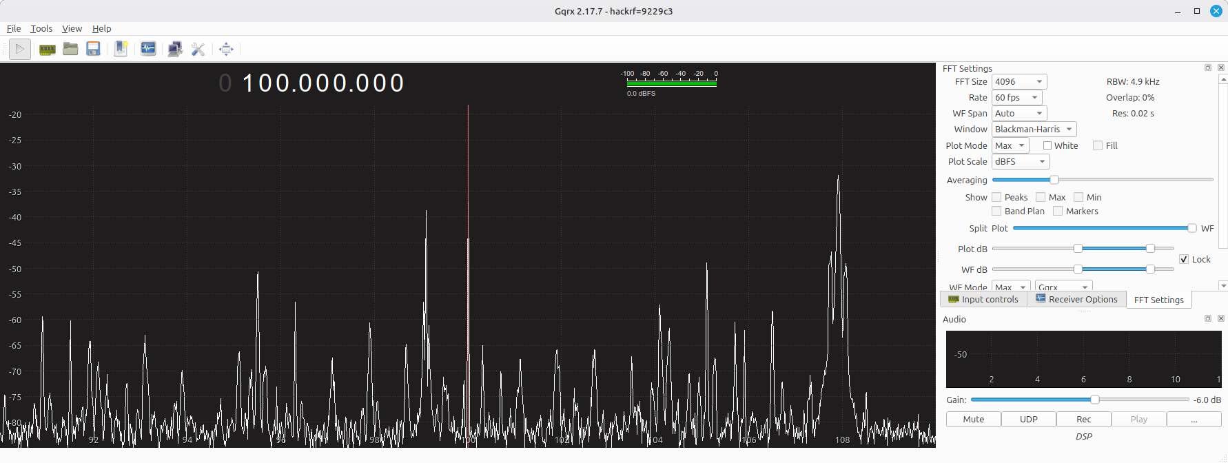
The manner in which your typical SDR program, such as GQRX or SDR++, provides a spectral display is that it tunes to a specific frequency, digitizes the energy within a certain span (based on the sample rate), calculates the FFT, and displays the magnitude of the FFT data. The RF tuner does not change; it's stays fixed at a specific frequency. The spectral display only shows the spectrum within +/- 1/2 of the sample rate within the center frequency. This is known as the instantaneous bandwidth or stare bandwidth.
Swept spectral displays allow for viewing spectral information over a larger amount of spectrum. Rather than being limited by the sample rate and RF front end bandwidths, the only limiting factor is the tuning range of the RF front end. It allows for the RF tuner to tune (or step) to different frequencies, collecting spectral information at each frequency, then stitching the spectral information together to form one, large display.
Understanding the Terms
As a sweeping spectral display may be new to many users, let's go through some basic terms. Some of these are standard; some are specific to this post. I'll be clear about which is which.
Sweep: (standard term) This term refers to the collection of spectral data from the lowest frequency to the highest frequency of a collected span. For example, if you want to see spectral data from 50 - 900 MHz, and your system collected such data, it would constitute one sweep. This may also be referred to as a "line" as the data will often be displayed on a spectrogram, where each sweep constitutes one line of the display.
Step: (standard term) This term refers to when a tuner will sit at a specific frequency while the radio collects energy within the limits of its sample rate and RF front end. A sweep will consist of one or more steps, with the number of steps determined by the step size of the SDR. For example, the HackRF step size is 20 MHz. A RTL-SDR operating with the spektrum program will use a 2 MHz step size. If both (hackrf_sweep and spektrum) are set to sweep the same frequency range, the HackRF will step in 20 MHz steps while the RTL-SDR will step in 2 MHz steps.
NOTE: The number of steps will be an integer value. Therefore, if the requested frequency range divided by 20 MHz provides some fractional value, it will be rounded up to the next integer value. For example, If the requested range is 200 - 410 MHz, this would be 10.5 steps. This will be rounded up to 11 steps, meaning that the system will cover from 200 - 420 MHz.
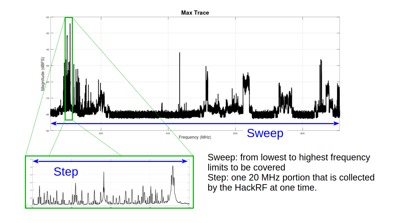
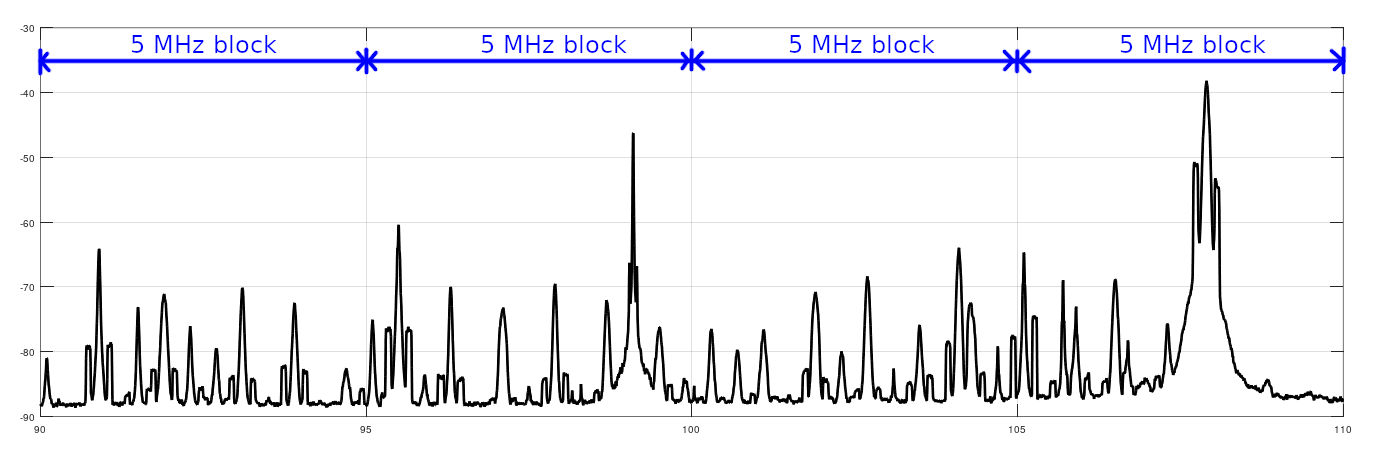
Block: (hackrf_sweep specific term) Within each 20 MHz step of the hackrf_sweep command, the spectrum will be divided into 4 equal blocks of 5 MHz each. This will be explained in much greater detail below.
A Basic Version of the Command
We'll be looking at hackrf_sweep straight from the command line. As my operating system is Linux (specifically, Linux Mint 22.3), I'm using the standard Linux terminal. At its most basic, the command requires a start frequency and stop frequency, both in MHz. Here's an example:
hackrf_sweep 100:200
where the 100:200 are the start frequency (100 MHz) and stop frequency (200 MHz). This command will output to the terminal (as that is the "stdout" or standard output, unless stated otherwise). This command on my system appeared as follows:
gary@main-Desktop:~$ hackrf_sweep -f 100:200
call hackrf_sample_rate_set(20.000 MHz)
call hackrf_baseband_filter_bandwidth_set(15.000 MHz)
Sweeping from 100 MHz to 200 MHz
Stop with Ctrl-C
2026-07-18, 18:34:29.430005, 100000000, 105000000, 1000000.00, 20, -32.74, -58.76, -44.46, -44.50, -43.10
2026-07-18, 18:34:29.430005, 110000000, 115000000, 1000000.00, 20, -50.12, -59.03, -80.70, -60.16, -59.98
2026-07-18, 18:34:29.430005, 105000000, 110000000, 1000000.00, 20, -37.86, -27.08, -17.78, -18.98, -33.22
2026-07-18, 18:34:29.430005, 115000000, 120000000, 1000000.00, 20, -62.95, -66.10, -65.01, -52.37, -53.89
2026-07-18, 18:34:29.430005, 120000000, 125000000, 1000000.00, 20, -65.02, -65.80, -63.95, -61.22, -65.61
2026-07-18, 18:34:29.430005, 130000000, 135000000, 1000000.00, 20, -60.30, -67.96, -65.93, -63.97, -62.58
2026-07-18, 18:34:29.430005, 125000000, 130000000, 1000000.00, 20, -66.52, -82.30, -68.13, -67.59, -65.52
2026-07-18, 18:34:29.430005, 135000000, 140000000, 1000000.00, 20, -67.55, -62.23, -58.45, -60.11, -63.21
2026-07-18, 18:34:29.430005, 140000000, 145000000, 1000000.00, 20, -57.04, -59.78, -67.50, -70.95, -68.57
2026-07-18, 18:34:29.430005, 150000000, 155000000, 1000000.00, 20, -68.40, -70.24, -64.13, -56.23, -57.58
2026-07-18, 18:34:29.430005, 155000000, 160000000, 1000000.00, 20, -62.48, -66.21, -70.81, -61.66, -74.70
2026-07-18, 18:34:29.430005, 160000000, 165000000, 1000000.00, 20, -62.62, -49.09, -45.55, -52.50, -66.79
2026-07-18, 18:34:29.430005, 170000000, 175000000, 1000000.00, 20, -63.64, -61.78, -62.81, -60.91, -59.61
2026-07-18, 18:34:29.430005, 165000000, 170000000, 1000000.00, 20, -56.42, -60.58, -91.62, -72.87, -64.85
2026-07-18, 18:34:29.430005, 175000000, 180000000, 1000000.00, 20, -59.67, -58.09, -58.18, -56.95, -55.16
...
Note that, even though I only let this run for an instant, it still managed to produce 384 lines of results, meaning it did 384/4 = 96 sweeps of that same 20 MHz span within that "instant".
While outputting to the terminal might be useful, for this post, I'm going to output to a file. To do that, we use the -r option, as follows:
hackrf_sweep 100:200 -r outputfile
where the -r outputfile means the data will be written as text to the file outputfile.
Looking at the Output
Take a look at the terminal output. This tells you a couple of things. These are:
- The output is in .csv (comma-delimited file) format. Hence, if you're not outputting in binary format (more on that later), the output will, by default, be in .csv format.
- The data is not written as straight spectral data. Each 20 MHz step covers four lines of the output file and is covered in linear form from start to finish (going from lines 1 to 5, 9, 13, etc). Within a step, the data is written in 5 MHz blocks. The blocks are not written straight from low to high. The center, two blocks are swapped.
Okay, so why are the center, two blocks swapped?
HackRF Hardware Review
Currently, there are two models of HackRF SDRs. These are the HackRF One, and the HackRF Pro. The HackRF One has an issue that is common to many SDRs, it has a DC feedthrough. This creates a spectral line, sometimes called a "spike", at the center of the spectrum.
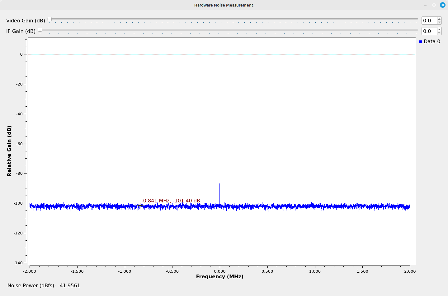
This DC feedthrough or DC "spike" is a part of the spectrum that is, essentially, useless. It would make spectral data more difficult to discern. To avoid this, the hackrf_sweep command does something a little different. The HackRF uses up to 20 MHz sample rate; the hackrf_sweep command is fixed at a 20 MHz sample rate, along with a 15 MHz bandwidth. A normal, sweeping spectrum analyzer would tune to a center frequency, digitize the spectrum, and display that spectrum. Because of the DC "spike", collecting the spectrum in a single collection would not work.
As explained above, the command hackrf_sweep operates on 20 MHz portions of spectrum at a time. The method by which it operates is as follows:[1].
- When it first starts running, calculate the minimum number of 20 MHz steps needed to cover the requested spectral range. As discussed above, the calculated number of steps will be an integer value.
- Start at the beginning frequency, and step up 7.5 MHz.
- Digitize the spectrum using a 20 MHz sample rate, and with a 15 MHz filter bandwidth.
- Calculate the magnitudes of the spectrum over the entire 20 MHz.
- Use only the spectral magnitudes from -7.5 to -2.5 MHz (a 5 MHz block given as block #1) and from 2.5 to 7.5 MHz (another 5 MHz given as block #3). This avoids the DC spike completely.
- Step up 5 MHz and repeat steps 2 - 4. This provides for blocks #2 and #4. This now covers the entire 20 MHz of the initial 20 MHz-step size.
- Step up 20 MHz and repeat steps 2 - 5.
- Continue repeating across each 20 MHz step required to cover the spectral range. All of the steps together to cover from its lowest frequency to the highest one is called a sweep.
Let's look, in graphical format, how data is collected in one 20 MHz step. Let's look at the spectrum from 90 - 110 MHz (20 MHz).
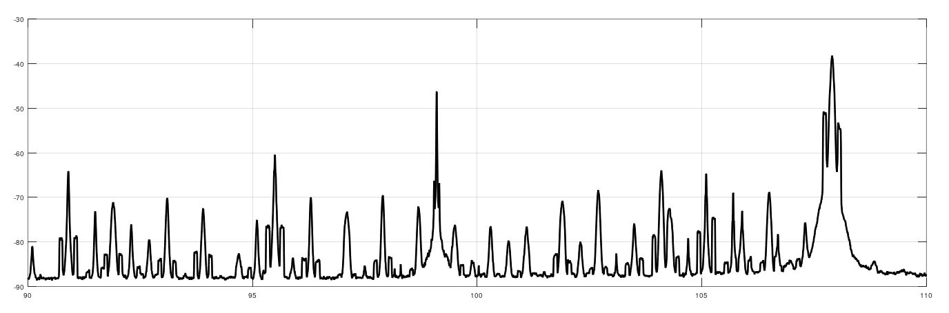
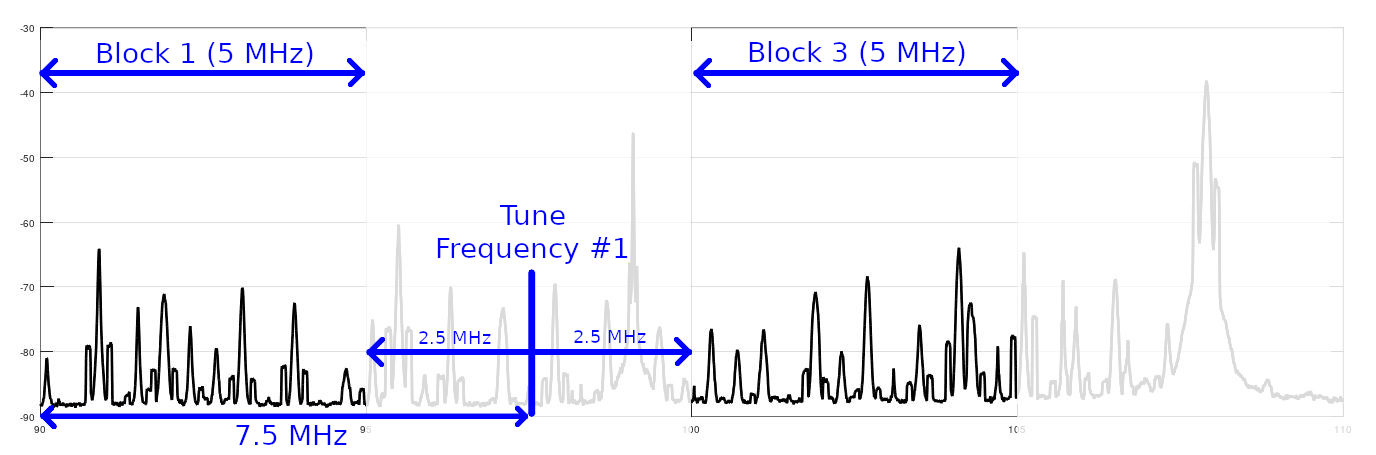
Using the low frequency limit (90 MHz, in this instance), it tunes 7.5 MHz above this lower frequency limit. It digitizes a 20 MHz swath of spectrum, then stores two 5 MHz blocks. One is 7.5 MHz below the tuned frequency, and the other is 7.5 MHz above the tuned frequency.
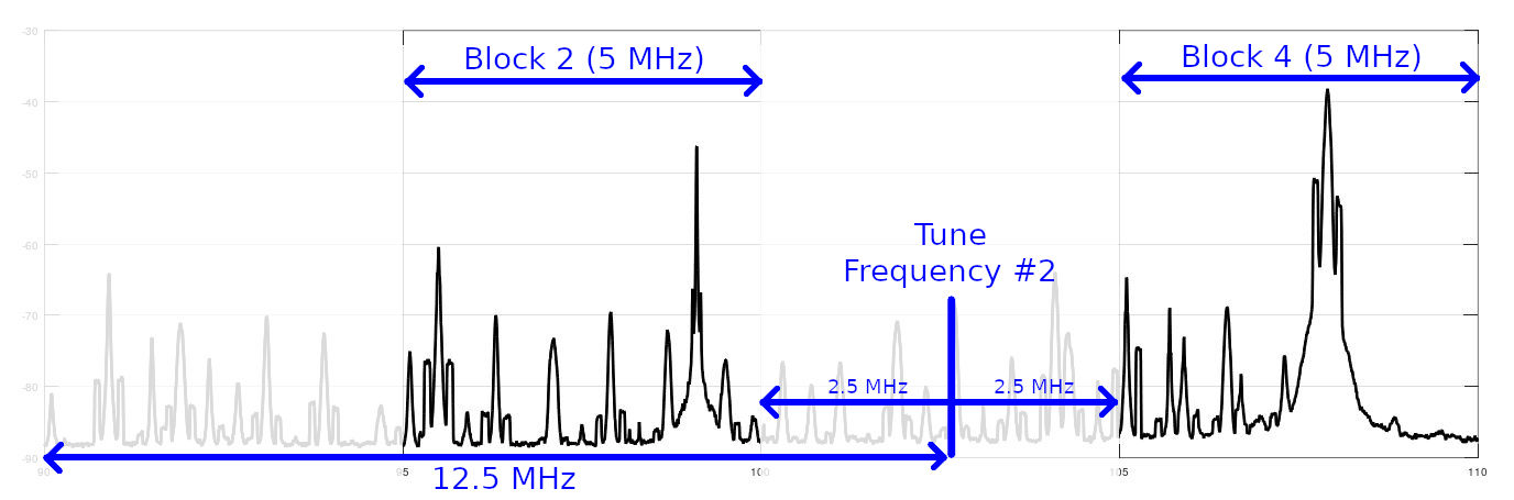
Once it completes collecting data in this two 5 MHz blocks, it steps up another 5 MHz (12.5 total from the lower frequency limit), digitizes a 20 MHz span, and collects two blocks of data similar to the first collection. However, because of the increased 5 MHz tuning from the first part, the two blocks cover the remaining 10 MHz spectrum of the original 20 MHz step.
When storing data in the default .csv format, one line of data (covering one 5 MHz block) will be as follows:
- Date
- Time
- Lower frequency, in Hz
- Upper frequency, in Hz
- Bin width, in Hz
- Number of bytes used to store spectral data, in binary format. Since this is 32-bit floating point (float32), the number of spectral points is this number divided by 4.
- (spectral data)
The data is stored in the same order in which it is collected. This is why looking at the basic output shows the data as follows:
2026-07-18, 18:34:29.430005, 100000000, 105000000, 1000000.00, 20, -32.74, -58.76, -44.46, -44.50, -43.10
2026-07-18, 18:34:29.430005, 110000000, 115000000, 1000000.00, 20, -50.12, -59.03, -80.70, -60.16, -59.98
2026-07-18, 18:34:29.430005, 105000000, 110000000, 1000000.00, 20, -37.86, -27.08, -17.78, -18.98, -33.22
2026-07-18, 18:34:29.430005, 115000000, 120000000, 1000000.00, 20, -62.95, -66.10, -65.01, -52.37, -53.89
Assuming the 5 MHz blocks covering one 20 MHz step are numbered 1 - 4, then the recorded blocks will be stored in the order 1-3-2-4. The center two blocks are swapped.
Collecting in Binary Format
The hackrf_sweep defaults to storing in .csv format, as explained above. However, it can also be stored in binary format. This uses the -B option in the command. The file format for binary storage is as follows:
- Unsigned 32-bit integer (uint32): the number of bytes in one 5 MHz block, minus the four bytes for this value.
- Unsigned 64-bit integer (uint64): the lower frequency limit, in Hz.
- Unsigned 64-bit integer (uint64): the upper frequency limit, in Hz.
- Spectral data magnitudes, in dBFS, written with 32-bit floating point values. The number of points can be calculated from the number of bytes in the 5 MHz block, minus 16 (for the two 8-byte frequency values) and divided by 4 (for the 32-bit floats).
Collecting data in this format has two advantages over the default .csv format. These are:
- The file will be smaller for the same data limits. The binary format doesn't have any of the formatting information as does the .csv format.
- The file will allow for faster processing, as it can be directly processed with standard programming languages.
I've created a Gnu Octave script that will process a binary file. It will display two spectral traces based on the collected data. One will be an average of all of the sweeps, and the other will be a maximum trace of all of the sweeps.
Command-line Options
The hackrf_sweep command has several options. We'll go through several examples showing these options.
Gain values: The first option is -a X to enable or disable the RF amplifier just past the antenna input. The possible values for X are 0 or 1. 0 means the amp is disabled; 1 means it is enabled. The next gain value is the IF gain, which uses the -l X option, where X can take on values between 0 - 40 dB in 8 dB steps. The final gain value is the baseband gain. This uses the -g X option, where X can take on values between 0 - 62 dB in 2 dB steps.
An example using these gain values is:
hackrf_sweep -f 100:200 -a 1 -l 8 -g 14 -B -r outputfile.bin
where:
- -f 100:200: this is the frequency range to be covered, from 100 - 200 MHz.
- -a 1: the RF amp is enabled
- -l 8: the IF gain is set to 8 dB.
- -g 14: the baseband gain is set to 14 dB.
- -B: the data will be stored in binary format
- -r outputfile.bin: this is the filename to which the data will be stored
Binwidth: The -w X option allows you to set the binwidth of the collected spectral data. This value will also set the size of the block feeding the FFT. Note that this value will typically not be the actual value used in the collection, although the actual value will be close. The method that hackrf_sweep uses to calculate the actual binwidth is as follows:
- Divide 5 MHz by the requested binwidth. For example, if the requested binwidth is 10 kHz, then 5 MHz / 10 kHz = 500.
- Calculate the integer value of this value. In this case, it's still 500.
- Add 1 to this value. Thus, the value would be 501.
- Use this value as the time record size of the FFT. This also means that the actual binwidth will be 5 MHz / 501 = 9980.04 Hz.
hackrf_sweep -f 100:200 -w 7500 -B -r outputfile.bin
where:
- -f 100:200: this is the frequency range to be covered, from 100 - 200 MHz.
- -w 7500: use the binwidth of 7.5 kHz. The actual binwidth, calculated as discussed above, will be ~7496.25 Hz.
- -B: output the data in binary format.
- -r outputfile.bin: this will be the output file name.
Number of sweeps: By default, the hackrf_sweep command will continually sweep the desired spectrum until the user manually intervenes. Another method is to use the -N X option, where X is an integer providing the requested number of sweeps.
hackrf_sweep -f 100:200 -w 5000 -N 100 -B -r outputfile.bin
where:
- -f 100:200: this is the frequency range to be covered, from 100 - 200 MHz.
- -w 5000: set the requested binwidth to 5 kHz. Given how it is actually calculated, it will be ~4995 Hz.
- -N 100: sweep across the spectrum 100 times.
- -B: output the data in binary format.
- -r outputfile.bin: output file name.
NOTE: The provided value is the binwidth, meaning the spacing between frequency points. It is not the resolution bandwidth (RBW). The hackrf_sweep command uses a Hann(ing) window, which has a NENBW of 1.5. This means that, if you want to calculate the RBW of the data collected, multiply the bindwidth by 1.5.
Wrapup
Let me wrapup with a few points of the hackrf_sweep command:
- The command operates on 20 MHz steps, minimum. This means that if you request low and high frequency limits that are less than 20 MHz apart, it will provide 20 MHz sweep, minimum.
- Within each 20 MHz step, the system is collecting data in 5 MHz blocks. These blocks are not recorded in straight 1-2-3-4 order. The reason is to avoid the typically large DC feedthrough of the HackRF One.
- The resulting data file can be quite large, especially if the sweep covers a large spectral range, if the binwidth is set low, and/or if the number of sweeps is large.
References
[1]: This explanation comes from the HackRF issues page on improving the hackrf_sweep command. It was provided by Github user "gozu42". While I've not read through the code myself to confirm these steps, they are consistent with the data provided by the hackrf_sweep command; therefore, I have no reason to doubt them.