Random Quote Board

Digital AM Demodulators

Gary Schafer, July 2021

Since I've taken such a deep look at the various forms of frequency demodulation, it's time to pay some attention to that other primary analog modulation method, amplitude modulation (AM). Rick Lyons put together a post on "Digital Envelope Detection". I'm going to build these different demodulators and see how well they work with Gnu Radio.

Amplitude Modulation Review

Let's do a quick review of amplitude modulation. It's one of the three types of sinusoidal modulation. The other two are frequency modulation (FM) and phase modulation (PM). The carrier, as always, is a sine wave. The envelope of a sinusoid is the difference between the maximum and minimum of the instantaneous amplitude of it.
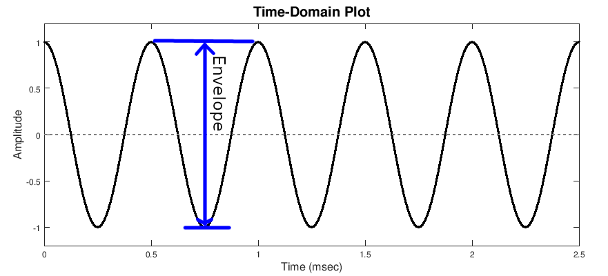
A sinusoidal wave in the time domain. An annotation shows that the envelope is measured from the top to the bottom of the waveform.
The envelope of a sinusoid is the difference between the instantaneous maximum and minimum of the sine wave.

Amplitude modulation varies this envelope, as shown below.
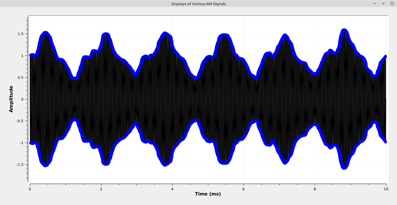
A black band indicating a modulated signal, with thick, blue lines tracing the top and bottom edge of the signal to indicate the modulating information.
AM signal showing the envelope (blue line on top and bottom of AM signal).

From a frequency viewpoint, AM carries the information in sidebands. When we look at the spectrum of AM signals, we have (up to) two sidebands, an upper sideband (one higher in frequency than the center frequency) and a lower sideband (one lower in frequency than the center frequency). Each sideband contains all of the information of the original signal. As a matter of fact, each sideband is the original signal, simply frequency translated up to a higher frequency and (possibly) frequency inverted.
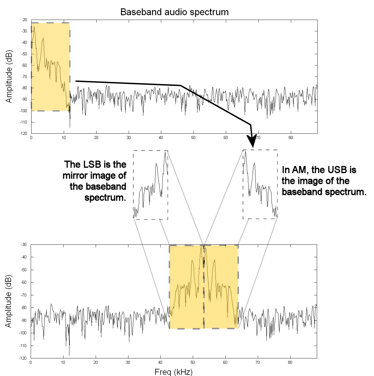
Diagram starting at the top with a spectrum of an audio signal. An arrow from that spectrum points down to a similar spectrum below, but annotated as upper sideband. To the left of that is the same spectrum, but mirror imaged and with the annotation lower sideband. At the bottom of the diagram is the spectrum of these two sidebands put together and annotated as double sideband.
Amplitude modulation translates the baseband signal to a higher center frequency. Unless it is processed in a special fashion before, such as by the Hilbert transform, the resulting signal will be a double sideband AM signal. This particular signal is a double sideband, suppressed carrier signal. We'll discuss that more below.

Amplitude modulation (AM) can be broken down based on two parameters. These are:

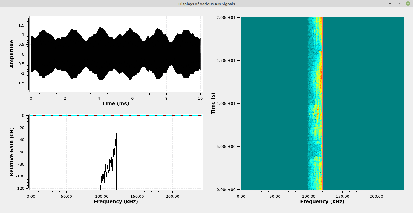
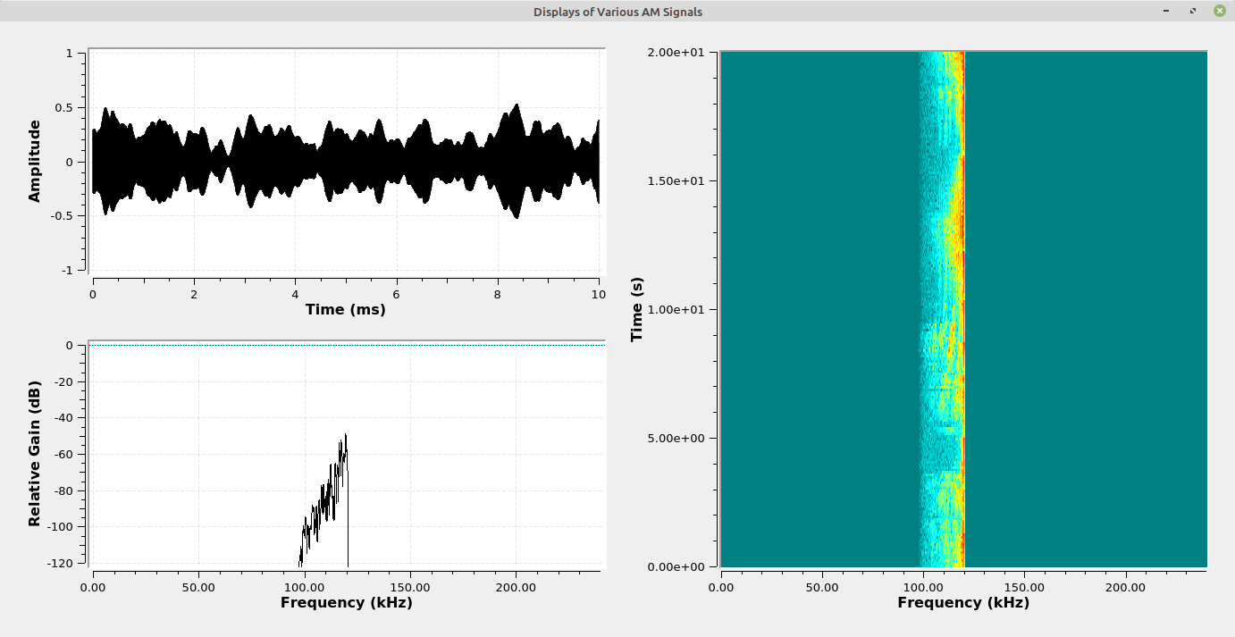
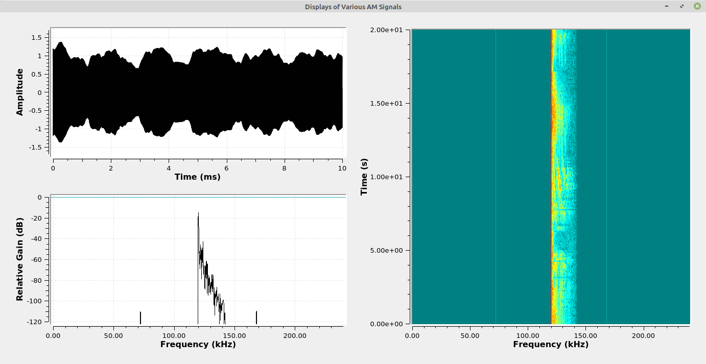
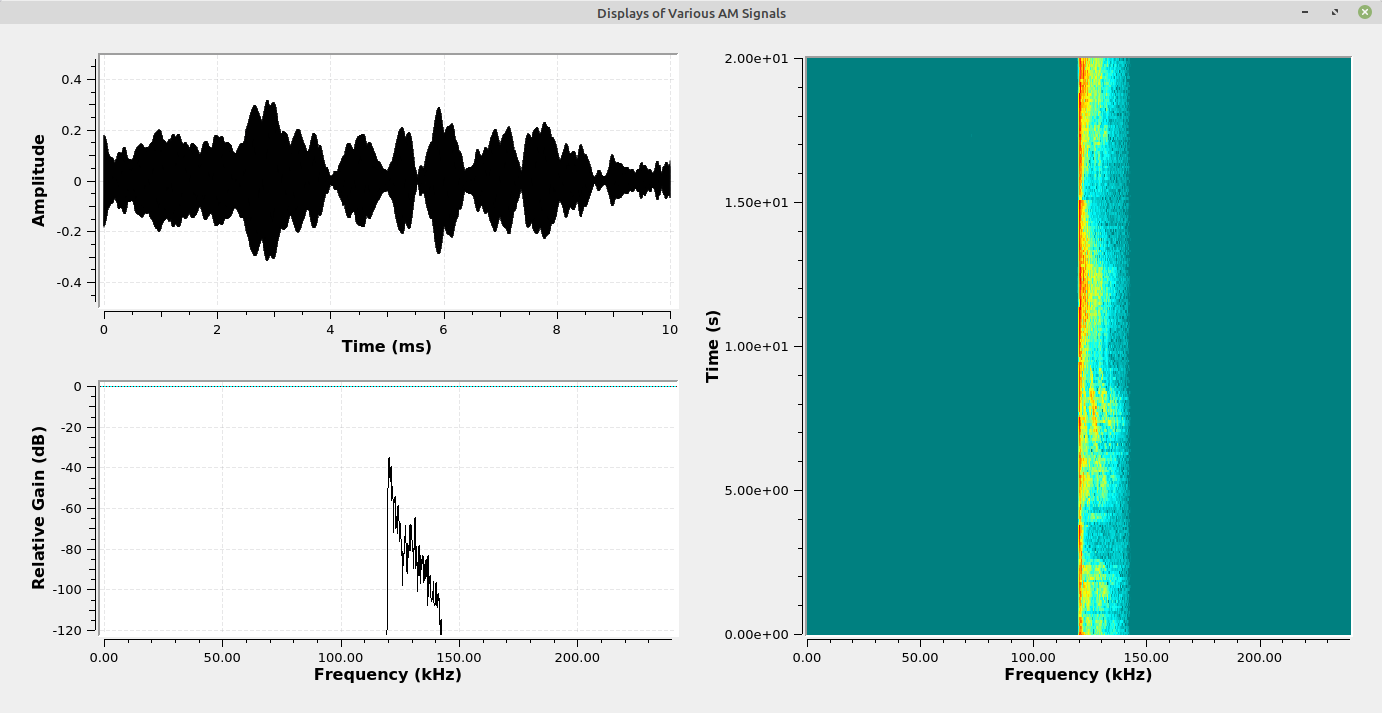
The following images show various facets of the different "flavors" of AM. For each image, the upper left display is the time domain showing the amplitude variation of the carrier. The lower left display is the spectral trace, while the right display is the spectrogram of the modulated signal.
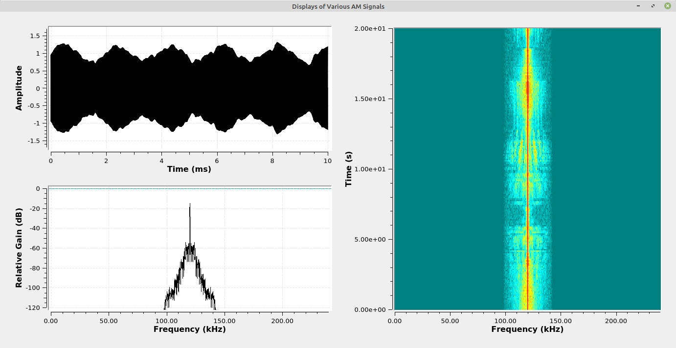
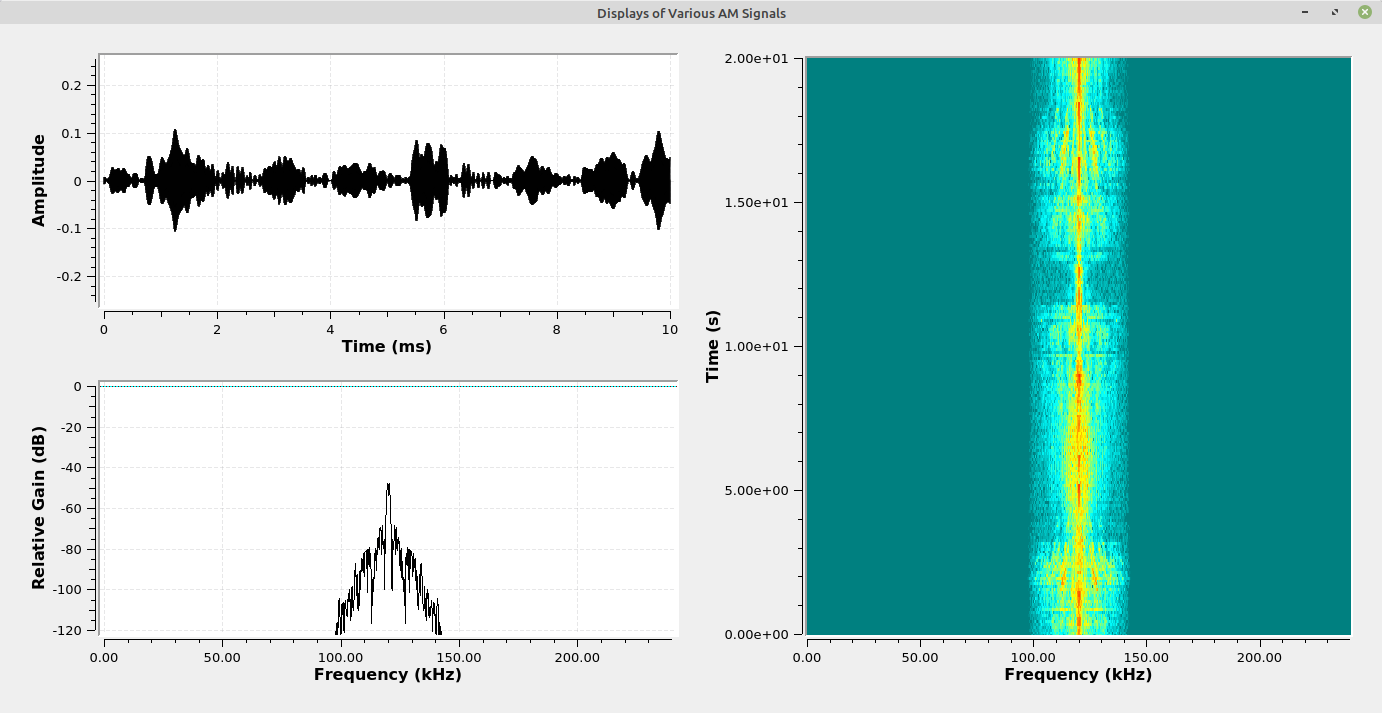
Screenshot of three displays, two on the left and one on the right. The one on the right extends from the top to the bottom of the screen. The two on the left are stacked one over the other, each taking up half of the height of the screen. The top left shows a waveform extending from left to right. The bottom left is a spectrum of a signal showing a small lump roughly bell shaped with a large thin line coming out at the peak and extending up near the top of the display. The display on the right is a color image showing a signal scrolling from top to bottom. In the middle of this signal is a red line showing the center carrier and on each side are varying sidebands, with each sideband a mirror image of the other.
Amplitude modulated audio signal using double sideband - full carrier.
Screenshot of three displays, two on the left and one on the right. The one on the right extends from the top to the bottom of the screen. The two on the left are stacked one over the other, each taking up half of the height of the screen. The top left shows a waveform extending from left to right. The bottom left is a spectrum of a signal showing a small lump roughly bell shaped with a small peak at the center. The display on the right is a color image showing a signal scrolling from top to bottom. On each side are varying sidebands, with each sideband a mirror image of the other.
AM audio signal using double sideband - suppressed carrier.
Screenshot of three displays, two on the left and one on the right. The one on the right extends from the top to the bottom of the screen. The two on the left are stacked one over the other, each taking up half of the height of the screen. The top left shows a waveform extending from left to right. The bottom left is a spectrum of a signal showing a small lump roughly triangular shaped that has been cut in half. Only the left half remains. A thin line sticks up from the peak. The display on the right shows a signal extending from top to bottom in the middle of the display. In the middle of this signal is a red line showing the center carrier and on the left side is a varying sideband.
AM audio signal using single sideband / lower sideband - full carrier modulation.
Screenshot of three displays, two on the left and one on the right. The one on the right extends from the top to the bottom of the screen. The two on the left are stacked one over the other, each taking up half of the height of the screen. The top left shows a waveform extending from left to right. The bottom left is a spectrum of a signal showing a small lump roughly triangular shaped that has been cut in half. Only the left half remains. The display on the right shows a signal extending from top to bottom in the middle of the display. The left side is a varying sideband.
AM audio signal using single sideband / lower sideband - suppressed carrier modulation.
Screenshot of three displays, two on the left and one on the right. The one on the right extends from the top to the bottom of the screen. The two on the left are stacked one over the other, each taking up half of the height of the screen. The top left shows a waveform extending from left to right. The bottom left is a spectrum of a signal showing a small lump roughly triangular shaped that has been cut in half. Only the right half remains. A thin line sticks up from the peak. The display on the right shows a signal extending from top to bottom in the middle of the display. In the middle of this signal is a red line showing the center carrier and on the right side is a varying sideband.
AM audio signal using single sideband / upper sideband - full carrier modulation.
Screenshot of three displays, two on the left and one on the right. The one on the right extends from the top to the bottom of the screen. The two on the left are stacked one over the other, each taking up half of the height of the screen. The top left shows a waveform extending from left to right. The bottom left is a spectrum of a signal showing a small lump roughly triangular shaped that has been cut in half. Only the right half remains. The display on the right shows a signal extending from top to bottom in the middle of the display. The right side is a varying sideband.
AM audio signal using single sideband / upper sideband - suppressed carrier modulation.
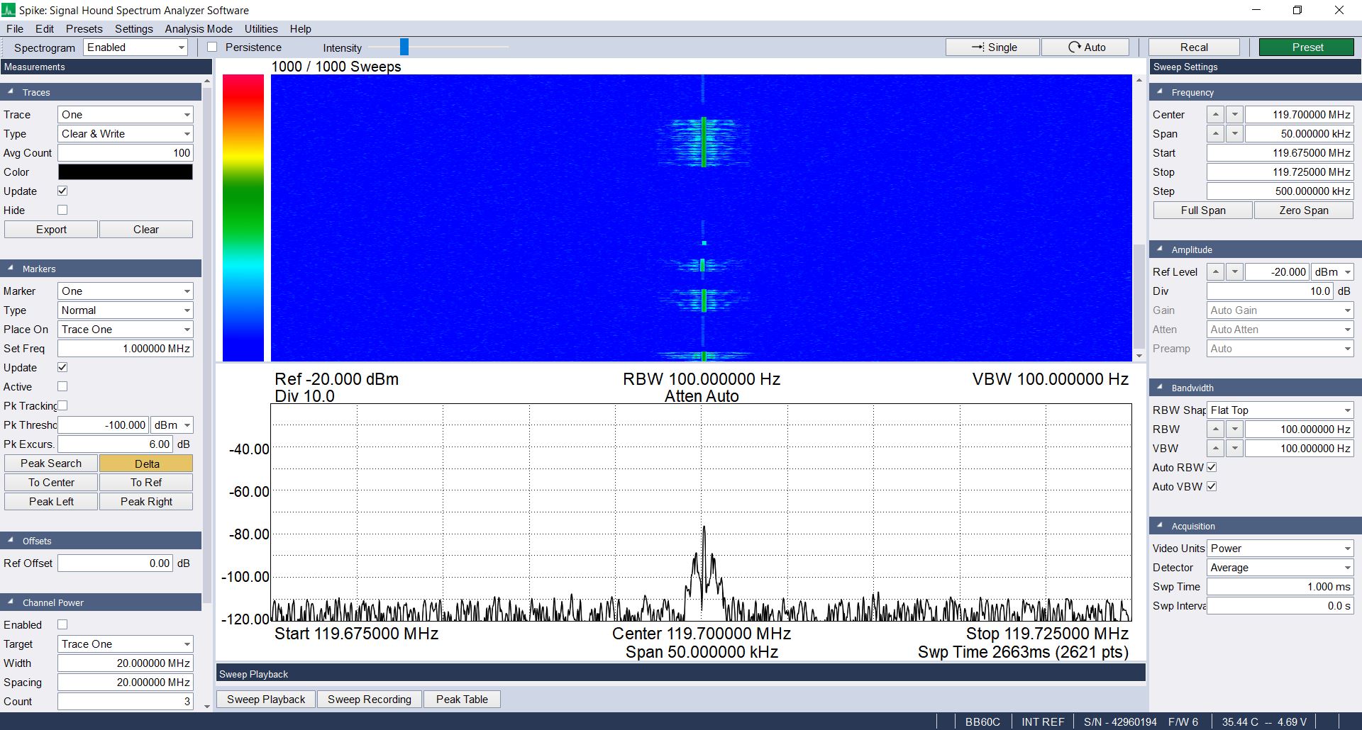
Screenshot of two spectral displays. The two displays take up the center of the screen with one on the top half and the other on the bottom half. The top half is a spectrogram. The bottom half is a spectral trace. In the center of the spectral trace is a roughly triangular shaped signal with a line sticking up from the center. The spectrogram shows a signal at the center that appears and disappears at several points as it traverses from top to bottom. On either side of the screen are controls.
This is the spectrum and spectrogram of an aircraft communications. Such communications have been double sideband - full carrier (DSB-FC) modulation for going on a century. (Image captured using Signal Hound "Spike" software and a BB60C SDR.)
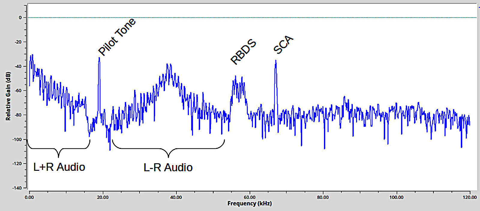
Spectral trace. The left end is roughly triangular shaped going from upper left to lower right. Where it stops, theres a line sticking straight up. Just to the right of that is another triangular-shaped signal that starts in the lower left, goes towards the upper right where it peaks, then extends back down to the lower right. This signal has the left half as a mirror image of the right half. Just to the right of this triangular-shaped signal is a narrower, roughly rectangular-shaped signal, with it higher than it is wide. At the top is a notch in the center. Just to the right of this is the a thin line sticking up. The rest of the display shows a noisy floor.
Baseband spectrum of a FM broadcast station. The "L-R Audio" signal, also called the "stereo signal", uses double sideband, suppressed carrier modulation. The FM receiver uses the "Pilot Tone" to demodulate this signal. Combined with the "L+R Audio" signal, this provides the receiver the capability to create separate left and right audio (stereo) signals.
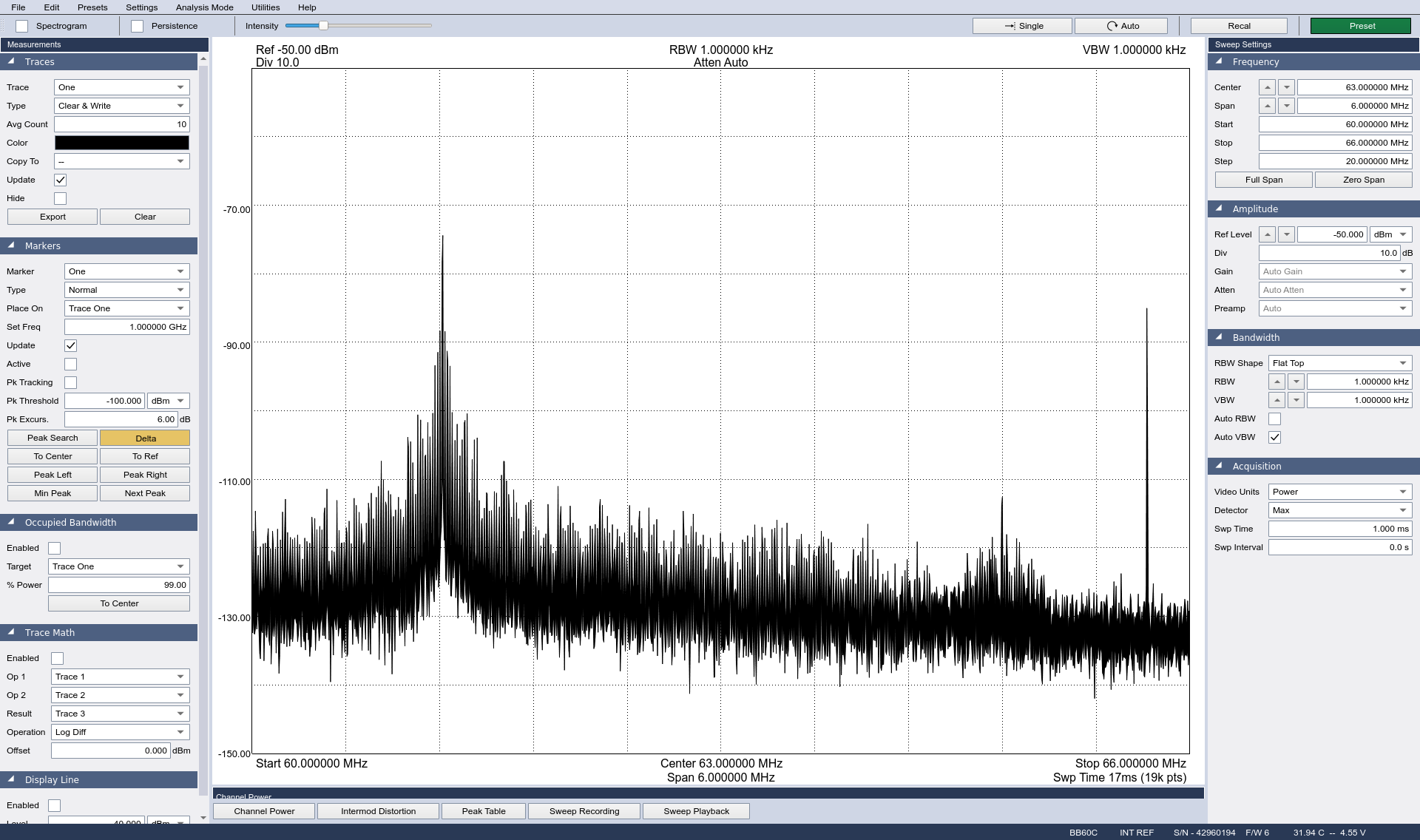
Screenshot of a spectral trace. Along the bottom is a noisy line. Near the left end, a signal comes up out of the noise and ends in a tall peak. The signal continues on the right as it descends towards the noisy floor. As it nears the right end, a small, triangular bump comes up, then drops back down. Almost at the right end, a line comes up out of the noisy floor. The right and left sides are covered with different controls.
A NTSC over-the-air signal. The large peak on the lower end of the spectrum is the video carrier. This was captured using a "RF modulator" to create a NTSC-like signal. An actual, broadcast NTSC signal used full carrier vestigial sideband (VSB) modulation. This modulator creates a full carrier double sideband signal. The large peak at the high end is the FM signal containing the audio synced with the video. The lower peak between these two is the chroma (color) signal.
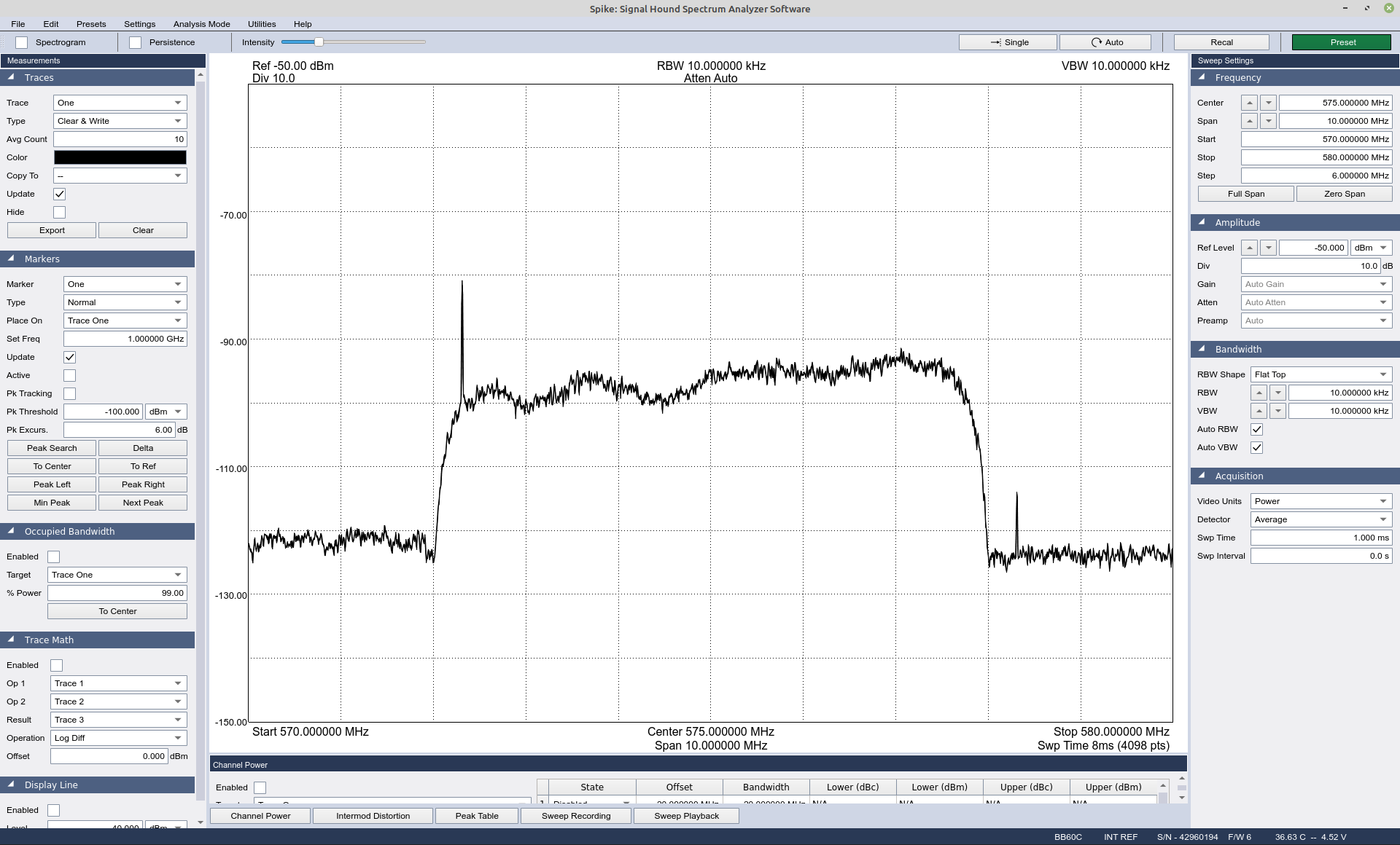
Screenshot of a spectral trace. The center of the screen shows the trace extending from the top to the bottom of the screen. Along the right and left ends are columns with controls. The trace shows a relatively flat line that rises up to a roughly rectangular shaped signal that has rounded corners on the top. Near the left end of this signal a line sticks up.
This is the spectrum of a ATSC transmission. The signal is also a vestigial sideband signal. The spectral line on the lower end of the signal spectrum is called a pilot. It's not a "carrier"; the carrier is actually suppressed. This pilot, however, can be (and is) used to recover the clock of the signal and allow it to be properly demodulated. The part of the spectrum to the left of the pilot is the vestige of the lower sideband. The part to the right is the upper sideband.

Amplitude Demodulation

Amplitude demodulation is the method we use to extract the original information from the modulated carrier. As the information signal varies the envelope, amplitude demodulation refers to extracting the envelope in order to recover the information.

General Methods of Demodulation

There are two, general methods for amplitude demodulation. These are noncoherent and coherent. Lyons's paper refers to this as asynchronous and synchronous, respectively. This refers to whether a sinewave in phase sync with the AM carrier is required. It's not required in the case of noncoherent / asynchronous, and required (sort of) for coherent / synchronous.
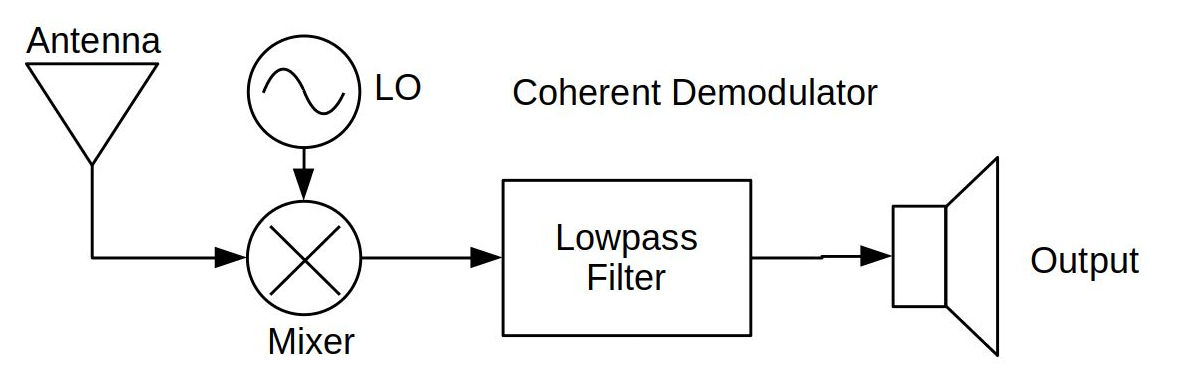
Block diagram showing a signal flow from left to right. A triangle in the upper left is marked antenna. An arrow traces from this down to a circle with an X in it marked mixer. Above this circle is another circle with a wavy line marked LO. An arrow extends from this circle to the lower one marked mixer. From the mixer, an arrow extends to the right to a rectangle marked lowpass filter. From the lowpass filter, an arrow extends to the right marked output.
Block diagram showing roughly how a coherent demodulator works. The "coherent" aspect comes from the fact that this demodulator requires the LO (local oscillator) to be in phase with the AM carrier. Otherwise, dropouts occur.
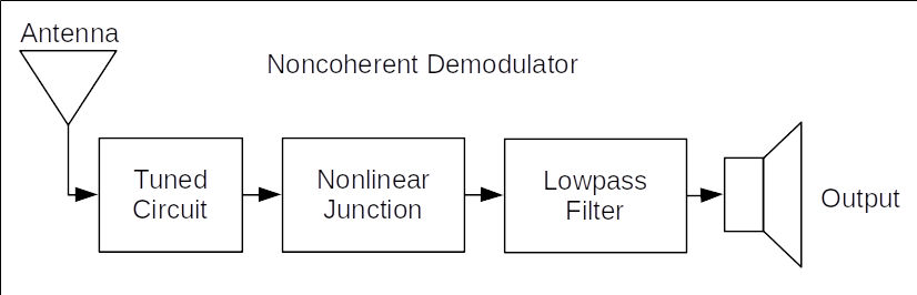
Block diagram showing a signal flow from left to right. The flow starts in the upper left with an upside down triangle marked as antenna. An arrow extends down and to the right of this to a rectangle marked tuned circuit. That continues to the right to a rectangle marked nonlinear junction, then to a rectangle marked lowpass filter, and finally to a symbol representing a speaker marked as output.
Block diagram showing how noncoherent demodulation works. For this to work, the AM signal must be full carrier. This demodulator uses that full carrier to demodulate the signal. A tuned circuit at the front end filters out all but the signal to be demodulated. The circuit typically uses some form of nonlinear circuit. This creates a mixing process in which the full carrier will be multiplied with the modulated signal. One product of that will be the information at baseband. The lowpass filter removes any higher frequency products, leaving just the baseband signal.

In his article, Lyons discussed several, different types of information that might be used. For example, he talked about amplitude shift keying (ASK, or amplitude modulation with digital bits as the information signal), basic analog audio, and medical electromyograms (EMG). For this post, I'm going to use simple audio signals, double sideband full carrier and suppressed carrier.

For all of the noncoherent demodulation methods, I'm going to use a double sideband full carrier signal.

Noncoherent Amplitude Demodulation

There are three general circuits for noncoherently amplitude demodulating a signal. All three perform the same basic function. They all remove the negative half-cycle of the modulated waveform. One circuit (half-wave rectified) simply removes the negative (or positive, depending on the polarity of the diode) portion of the time domain waveform. The other two circuits (full-wave rectified, squaring) convert the negative to positive amplitudes.

In this case of a full carrier system, this is not a problem. As seen below, with noncoherent demodulation, we've not affected the information. Noncoherent won't work with suppressed carrier due to the fact that the rectification process (regardless of how it is performed) will distort the original information signal.
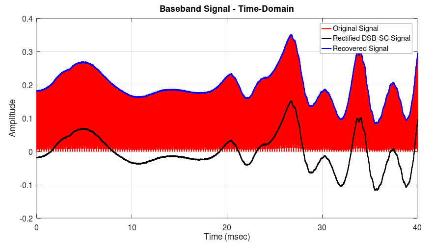
Time domain trace with time on the horizontal axis and amplitude on the vertical axis. A red band extends across the display, with the low end reaching zero, while the upper part is wavy with varying maxima and minima. A blue line traces the top of the red band. A black line that matches the blue line runs from left to right, but is centered around zero.
This shows a double sideband full carrier signal after it has been rectified (in red). The recovered signal (blue) is identical to the original signal (black), but with a DC offset. The DC offset is due to the full carrier. Due to this DC offset, the information signal (blue) is not affected by the rectification process on the modulated waveform (red).
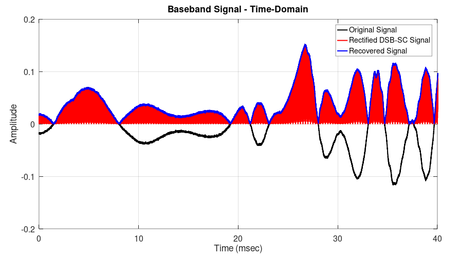
Time domain trace with time on the horizontal axis and amplitude on the vertical axis. A red band extends across the display, with the low end reaching zero, while the upper part is wavy with varying maxima and minima. This is a much thinner band of red than the previous screenshot. This band of red is centered vertically around zero. A blue line traces the top of the red band. A black line runs from left to right that is also centered around zero. This time, the blue line doesn't always match the black line since sometimes the blue line is always above zero, while the black line will occasionally drop below zero. When that happens, the black and blue lines are mirror images vertically of each other.
This shows a double sideband suppressed carrier signal in the time domain after it has been rectified (in red). The recovered signal (blue) is a distorted version of the original signal (black). Because of the suppressed carrier, there is no DC offset to keep the envelope away from crossing the zero line. This means that the rectification process will not only rectify the modulated waveform (red), but also the information signal. Thus, noncoherent does not work with suppressed carrier signals.

Half-wave Rectified Envelope Detection

Lyons's first demodulation method is the "Asynchronous Half-Wave Envelope Detection". The first such receiver used a crystal to create a diode. This method led to one of the first, massed produced AM receivers. Those were "cat's whisker" receivers, a form of crystal receiver. These receivers started with an external antenna, a loop of wire that was used to tune the receiver, a nonlinear junction (the "cat's whisker" combined with a crystal) that acted as a diode, and a headphone output.
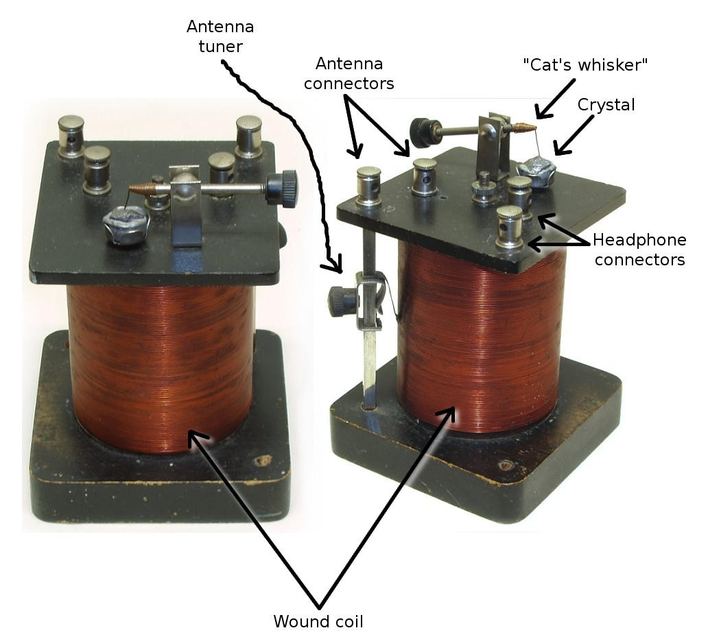
Image of two cylinders roughly 4 cm (1.5 inches) in diameter, each one roughly 8 centimeters (3 inches) high. The cylinders are wrapped in copper colored wire from top to bottom. The bottom of each cylinder is a black, square base roughly 5 cm (2 inches) on a side.  The top is a similar square, black shape but only 6 millimeters (0.25 inches) thick. On the top of the top square are several silver-colored posts, some with holes in them and one taller one that has a horizontal pin. At the end of the pin is a thin wire extending down to a small cap on the top of the top, black square.
"Cat's whisker" receiver. Note that there were many different such receivers. A "cat's whisker" is a generic name; it does not apply to one, specific receiver. As this is a noncoherent demodulator, we can match each section to the block diagram above. An antenna would be attached to the noted connectors. The wound coil worked as part of a tuned circuit to tune in the signal-of-interest. The "cat's whisker" is the nonlinear element. The final block, the lowpass filter, is not shown. It's the human ear. As the ear does not work with frequencies above 15 - 20 kHz, it filters out all of the higher frequency components.(Photo credit courtesy of Radiolaguy.com, with my annotations. Used with permission.)

This first circuit is one of the first nonlinear demodulation methods. The crystal acts as a diode, which half-wave rectifies the modulated signal. The spectrum (below) shows a baseband signal (the original information), the original, modulated signal, plus copies of the signal at even harmonic frequencies.
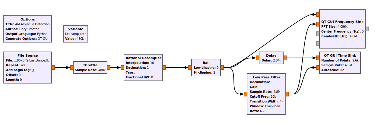
Block diagram for signal processing. The signals flow from left to right. The diagram consists of four squares ordered from left to right, at which point the signal flow splits between three display blocks. The first block is a file source, then processes through a throttle, followed by a resampler, then a block marked rail. From here, the signal flow splits into three legs, with the top leg being displays in a spectral display, the middle leg going into a time sink, and the lower leg being filtered then going into the same time sink.
Gnu Radio graph of the half-wave rectified receiver. The Gnu Radio block "Rail" acts as the diode (nonlinear circuit). The resulting spectrum shows the baseband signal, the original signal, plus even-numbered harmonics of the original signal. The lowpass filter removes all but the baseband signal.
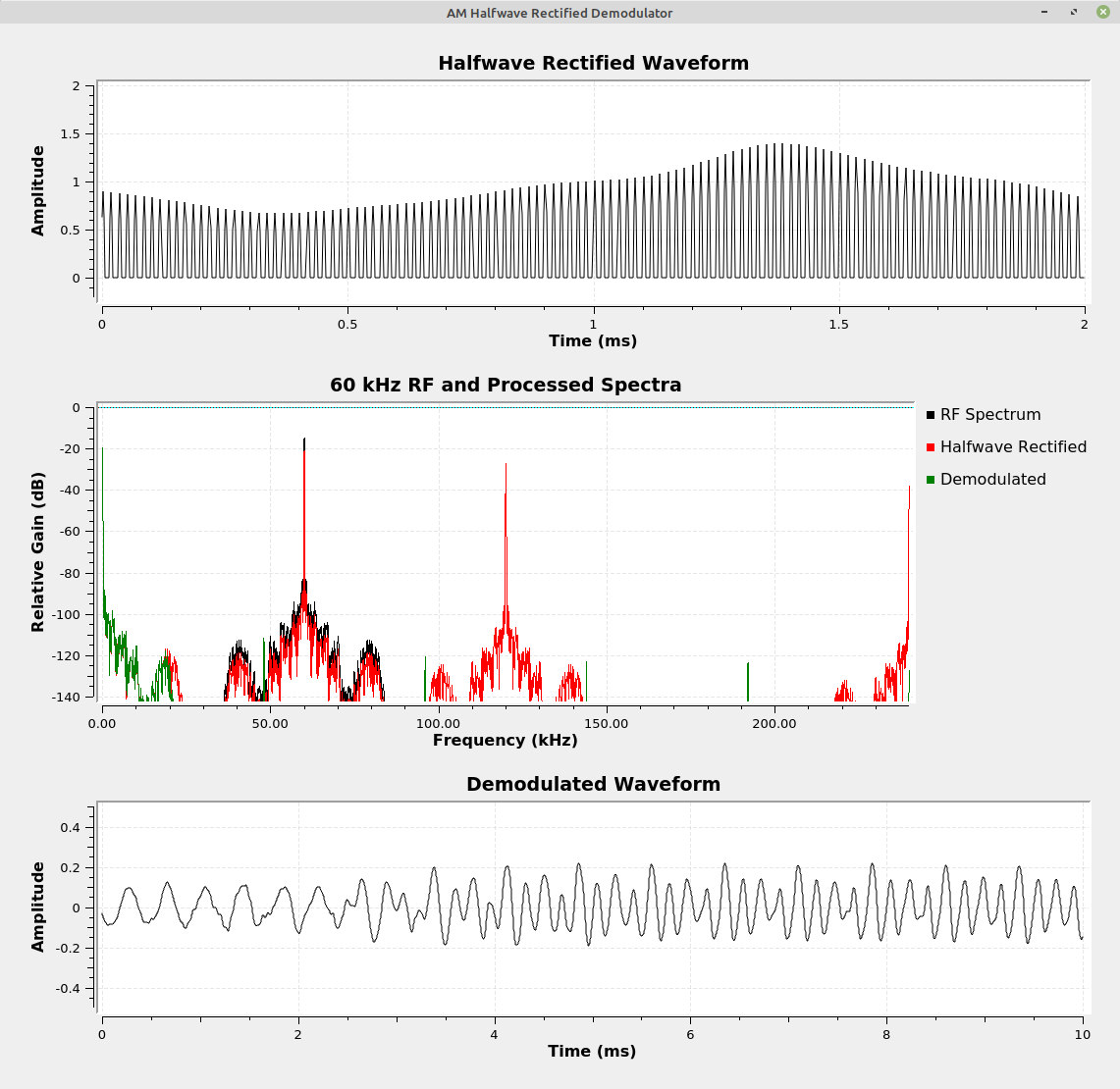
Three displays ranged from top to bottom. Each display takes up roughly 1/3 of the screen vertically. The top display shows a sinusoidal signal whose portion below zero has been removed. The center display shows the spectrum with several signals present. The bottom display shows a roughly sinusoidal waveform with the amplitudes varying.
This shows the time domain (top) and frequency domain (center)of the rectified signal. The bottom is the demodulated signal. The spectrum shows the modulated signal in black and the rectified signal in red. The lowpass filtered signal is shown in green.

Full-wave Rectified Envelope Detection

A problem with the half-wave rectified receiver is that it essentially throws away half of the signal. To correct this, we can use a full-wave rectified circuit. It's typically a diode bridge consisting of four diodes. The diodes create a circuit in which the output will be a positive signal regardless of whether the input is positive or negative. In the digital domain, a full-wave rectified receiver can be created using the "Abs" function, as seen below. In an analog system, this would probably be a diode rectifier circuit in which two sets of diodes would provide for the full rectification of the modulated waveform.
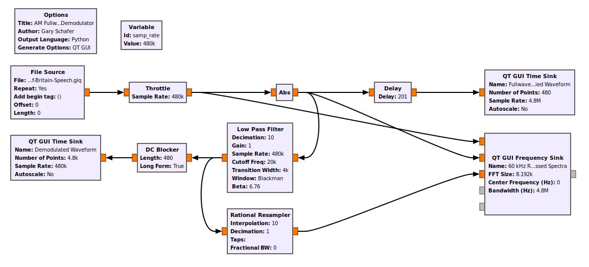
Block diagram for signal processing. The signal flows from left to right. The diagram consists of multiple rectangular blocks connected from left to right along the top, then half-way over, four blocks lower down process the signal from right to left. The blocks provide input from a file (first block on the left), followed by blocks for maintaining clock (throttle) and calculating the absolute value of the signal. The lower blocks filter the signal, remove DC, and then display the signal on a time domain display. The remaining top blocks display the time domain and spectrum of the signal.
The full-wave rectified receiver replaces the "Rail" block with the "Abs" block. This rectifies the complete wave, as opposed to only half of it with the "Rail" block.
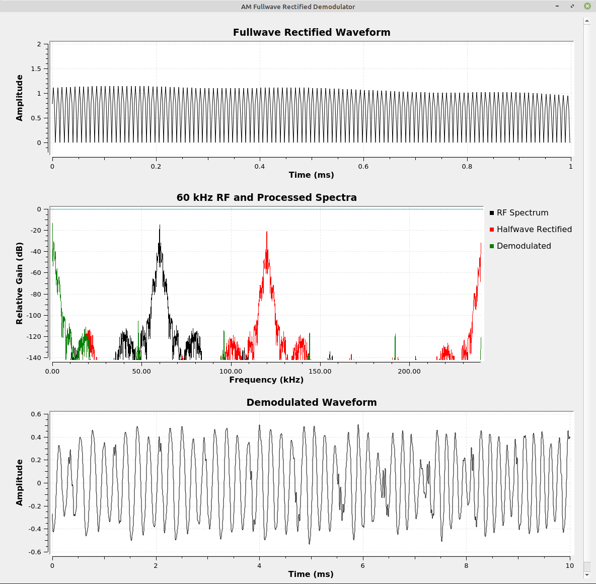
Three displays ranged from top to bottom. Each display takes up roughly 1/3 of the screen vertically. The top display shows a sinusoidal signal whose portion below zero has been flipped so that it is now positive. The center display shows the spectrum with several signals present. The bottom display shows a roughly sinusoidal waveform with the amplitudes varying.
This shows the full-wave rectified waveform in the time domain (top) and spectrum (center). Note that the spectrum shows the baseband signal, and even harmonics of the fundamental. Unlike the half-wave rectified signal, the full-wave rectified does not show the original signal. The bottom graph shows the demodulated output.

Squared Rectified Envelope Detection

If you look at the spectrum of both the half-wave and full-wave rectified circuits, you'll see signals at the top end of the spectrum. Both the half-wave and full-wave circuits create harmonics that run off to... infinity.
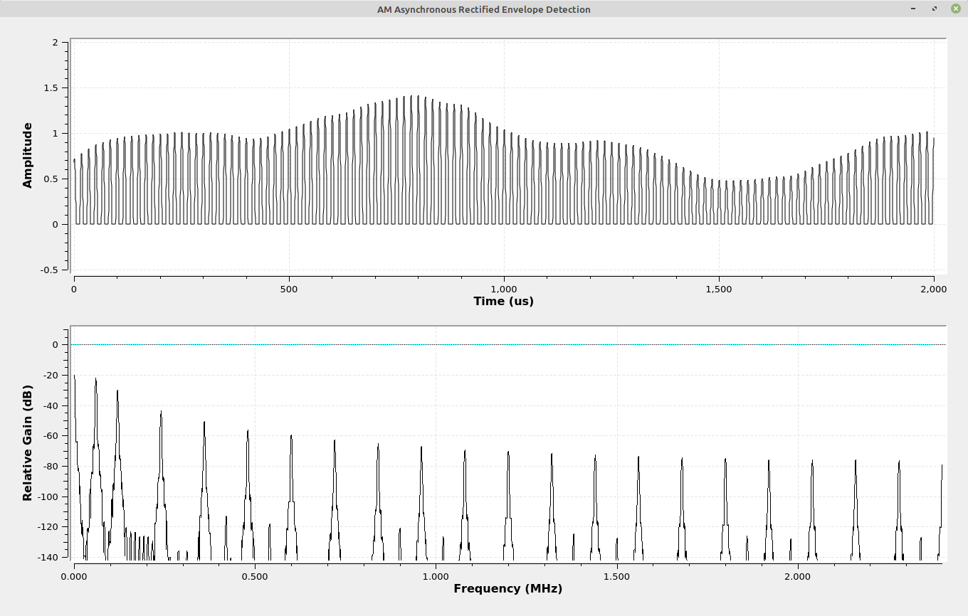
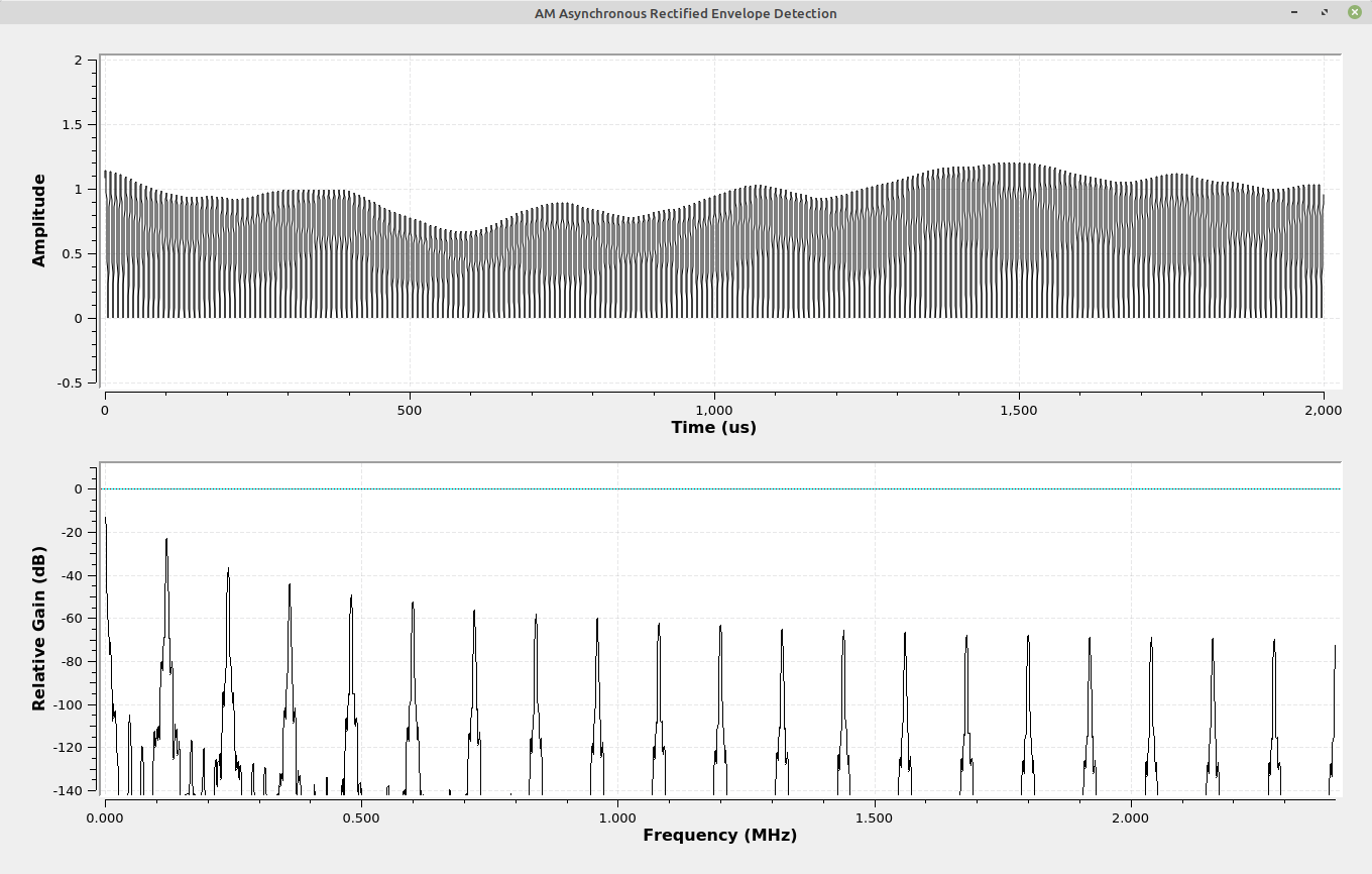
Time domain and spectrum of half-wave rectified AM signal. This shows how the spectrum consists of the original signal, plus harmonics of the signal that theoretically go out to infinity. Eventually, regardless of the sample rate, the harmonics will create aliasing in the signal.
Time domain and spectrum of a full-wave rectified AM signal. This spectrum is similar to the half-wave rectified version, with the exception that the signal at the original frequency is not present. Otherwise, we still have harmonics that go out to infinity, which creates aliasing.

This is not a problem for the original, analog circuits. It doesn't work so well in the digital realm. Such harmonics will create aliasing. This next circuit solves this problem. It uses the simple means of squaring the signal (multiplying it by itself). The result will be a baseband signal and a signal at twice the frequency. There will be no higher order harmonics than the second harmonic. Hence, no aliasing.
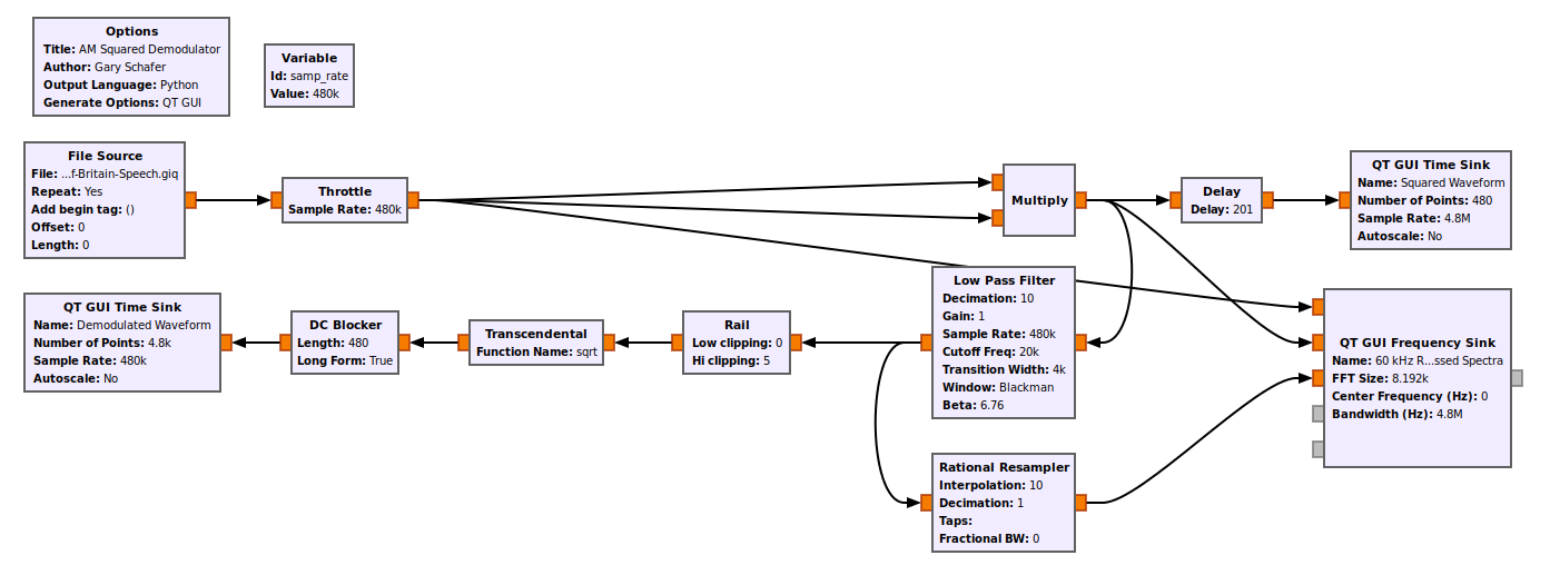
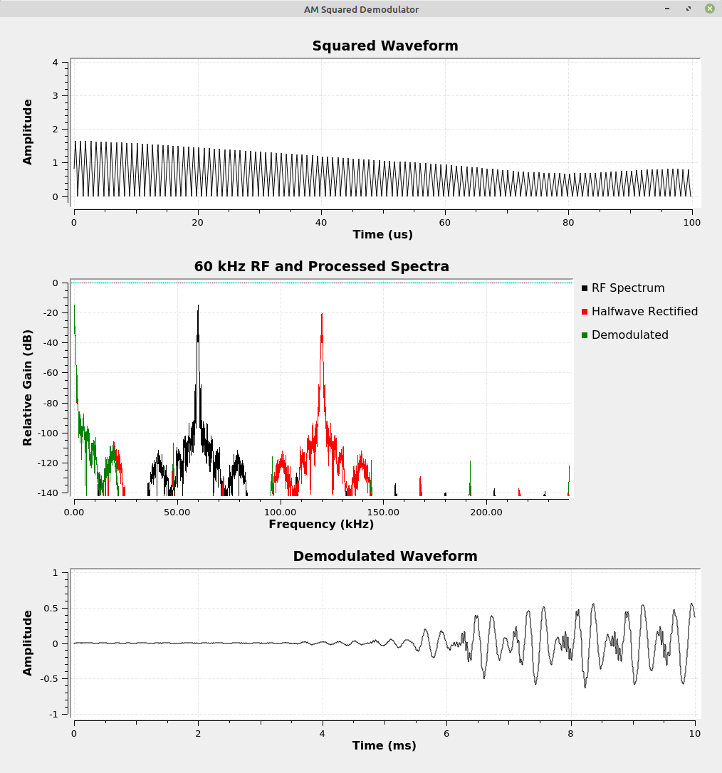
This is the graph for the squared demodulator. The time domain will be similar to the full-wave rectified signal. However, the resulting signal only creates a second harmonic, but it does require a square root circuit to keep the amplitudes at the proper levels.
This shows the squared signal in the time domain (top) and spectrum (center). Note that the squared spectrum only has the second harmonic and baseband signal. The bottom shows the demodulated waveform.

The only issue with this circuit is that the squaring operation requires a de-squaring (square rooting?) operation in order to bring the amplitude levels back to normal. For this operation, I used the "Transcendental" block to calculate the square root. Note that there's a "Rail" block just before the "Transcendental" block with the "sqrt" function. The reason for the "Rail" block is to prevent any values less than 0. The "sqrt" function cannot handle negative values. I discovered that, when the graph first starts running, there could be negative values that occur. The "Rail" block prevents that.

Envelope Detection with Complex Signals

Up til now, all of the signals and processing have used real, not complex, signals. Lyons's next, few circuits change that. While each circuit starts with a real signal, the signals are converted to complex. The complex conversion takes one of two forms:

  1. Hilbert Transform: The first method simply uses the Hilbert transform to convert the signal from real to complex. This keeps the signal at the same center frequency, but eliminates the negative frequency signal. The first "Asynchronous Complex Envelope Detection" and the "Asynchronous Complex Square-Law Envelope Detection" are of this type.
  2. Quadrature Demodulator: The second method is the traditional method to convert any signal from real to complex. It uses a pair of sinusoid oscillators, 90 degrees out of phase with each other, followed by a lowpass filter for each, to convert the signal into complex. The difference from the Hilbert transform is that, in this case, the signal will be frequency shifted by the frequency of the oscillators. The second "Asynchronous Complex Envelope Detection" is of this type.
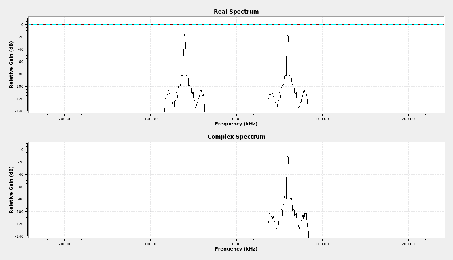
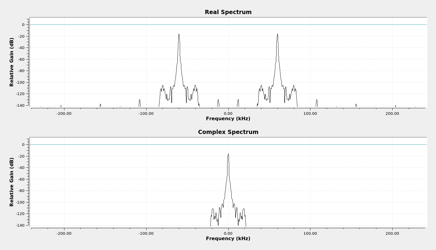
This is the real vs complex spectrum after the real signal has been converted to complex using the Hilbert transform. The center frequency does not change; the negative frequency component is simply eliminated.
This is the real vs complex spectrum after the real signal has been converted to complex using a quadrature demodulator circuit. In this case, the signal has been translated to baseband.

What I noticed looking at the block diagrams for the various asynchronous (noncoherent) envelope detection methods is that they're similar, if not the same, as those for the real signals. The difference is that you have to do each of them twice, one each for the real and imaginary component.

Asynchronous Complex Full-Wave Envelope Detection

This first complex system makes use of the Hilbert transform to translate the signal from a double-sided real signal into a single-sided complex signal. It takes each leg of the complex signal, both real and imaginary, and performs full-wave rectification on each.
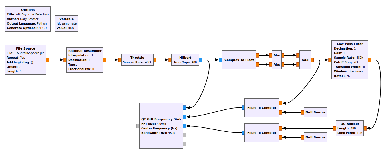
Graph for turning the real AM signal into a complex signal using the Hilbert transform, then performing envelope detection by performing full-wave rectification on each branch of the complex signal (real and imaginary).
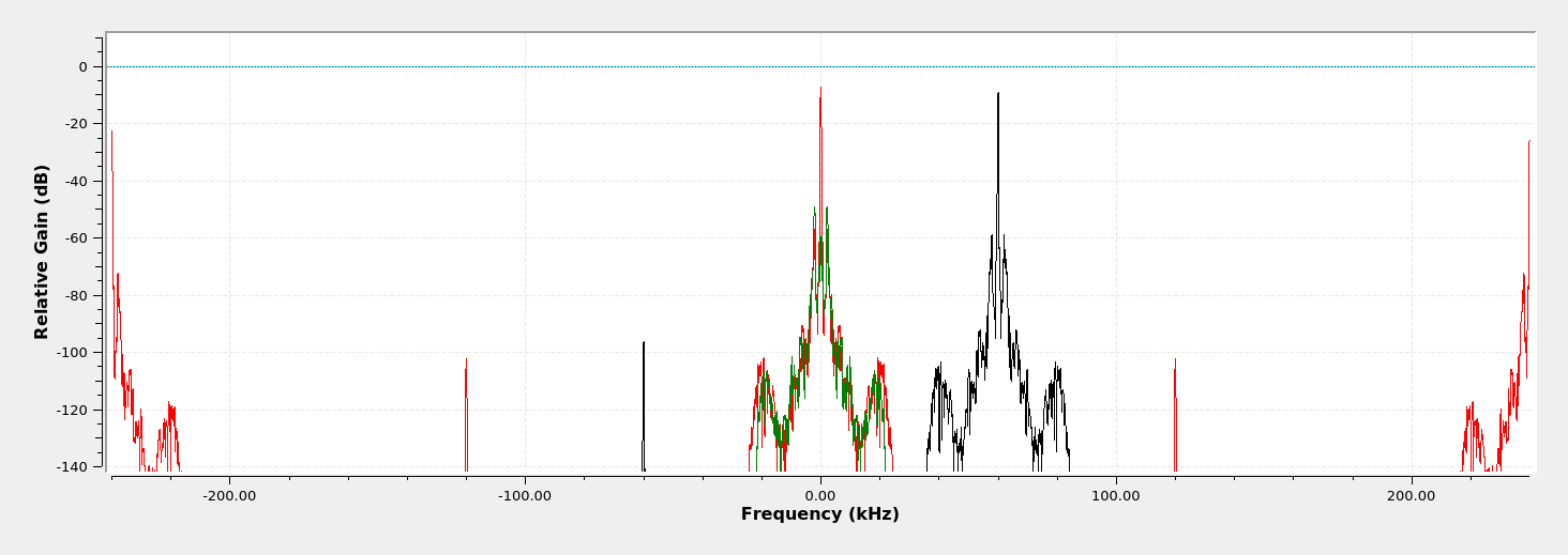
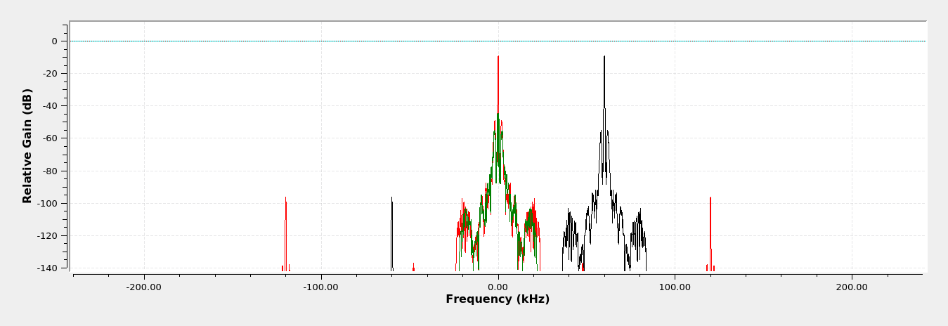
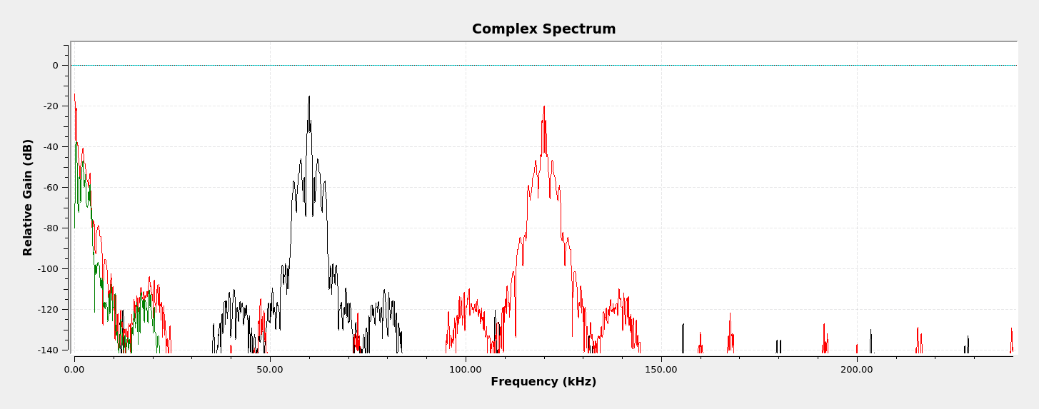
This is the complex spectrum of the signal showing the baseband signal after demodulation (green), the modulated signal after being passed through the Hilbert transform (black) and the signal after the full-wave rectification process (red).

This is where we see a difference between the real and complex operations. In the rectification of the real signal, the spectrum showed even numbered harmonics (2, 4, 6, etc). The spectrum of the complex rectified only shows every 4th harmonic (4, 8, 12, etc).
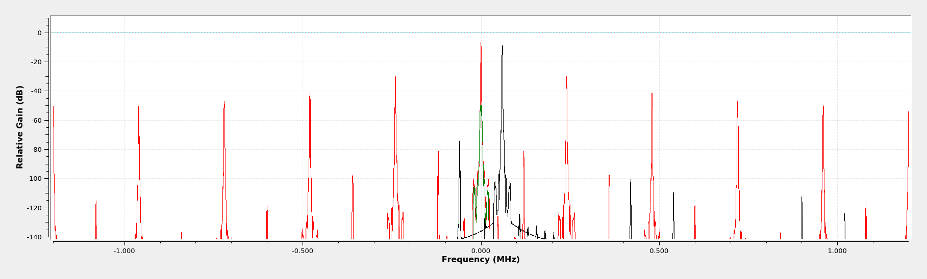
This is the spectrum of a complex full-wave rectified signal. It only shows every 4th harmonic. This is different from a real rectified (half-wave or full-wave) signal, which shows every even-numbered harmonic (2, 4, 6, etc). The black signal is the spectrum of the original AM signal (DSB-FC). The red is the signal after full-wave rectification. The green is the baseband signal after being lowpass filtered.

Asynchronous Complex Squared Envelope Detection

This graph is similar to the last one. The real signal is first passed through the Hilbert transform in order to create a complex signal. The real and imaginary components of the complex signal are squared individually, then the products added together. The result is a signal at baseband plus a signal at twice the original modulated frequency. The lowpass filter removes the signal at twice the frequency, leaving the information signal.
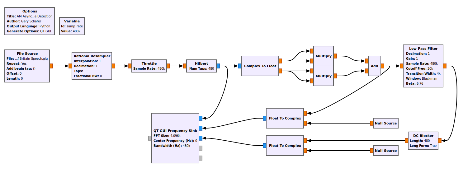
Graph for the complex and squared circuit. In effect, this calculates the magnitude squared of the complex signal. This graph is missing a square root function to put the amplitudes of the baseband signal back to normal amplitudes.
This is the spectrum for the magnitude squared signal. The result is only the baseband signal. This could be used without a lowpass filter. However, Lyons's article explicitly states, "However, I have learned this only to be true for noise-free signals! In practical real-world applications the lowpass filter I've included ... is necessary."

The graph above implements the magnitude squared function. It turns out that the "Complex to Mag" block will also work. Further, it provides the proper amplitudes.
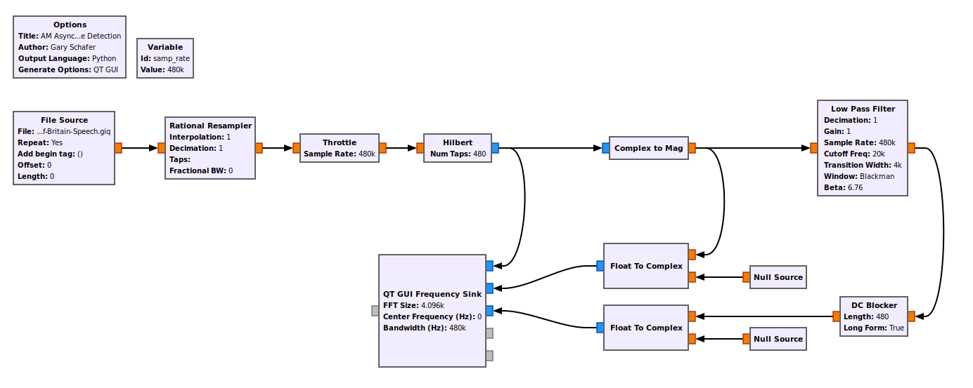
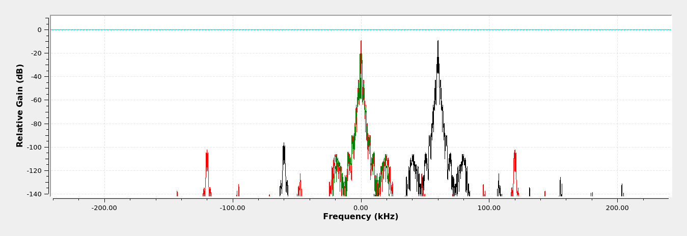
Graph using the "Complex to Mag" block. This calculates the actual magnitude (not just the magnitude squared) of the AM signal. The result is similar to that of the magnitude squared graph.
Complex spectrum of the "Complex to Mag" block on the complex AM signal. The result is the same as the previous graph, but without requiring a separate square root block. It also includes a lowpass filter, though its not theoretically required. Lyons recommends using one, though.

Asynchronous Quad Demod Complex Squared Envelope Detection

This last one is interesting. It turns the real signal into a complex signal using a quadrature demodulator. This consists of two sinewave generators that are in sync, but are 90 degrees out of phase. These sinewave signals are mixed with the modulated signal. After this, they're squared, added and lowpass filtered.
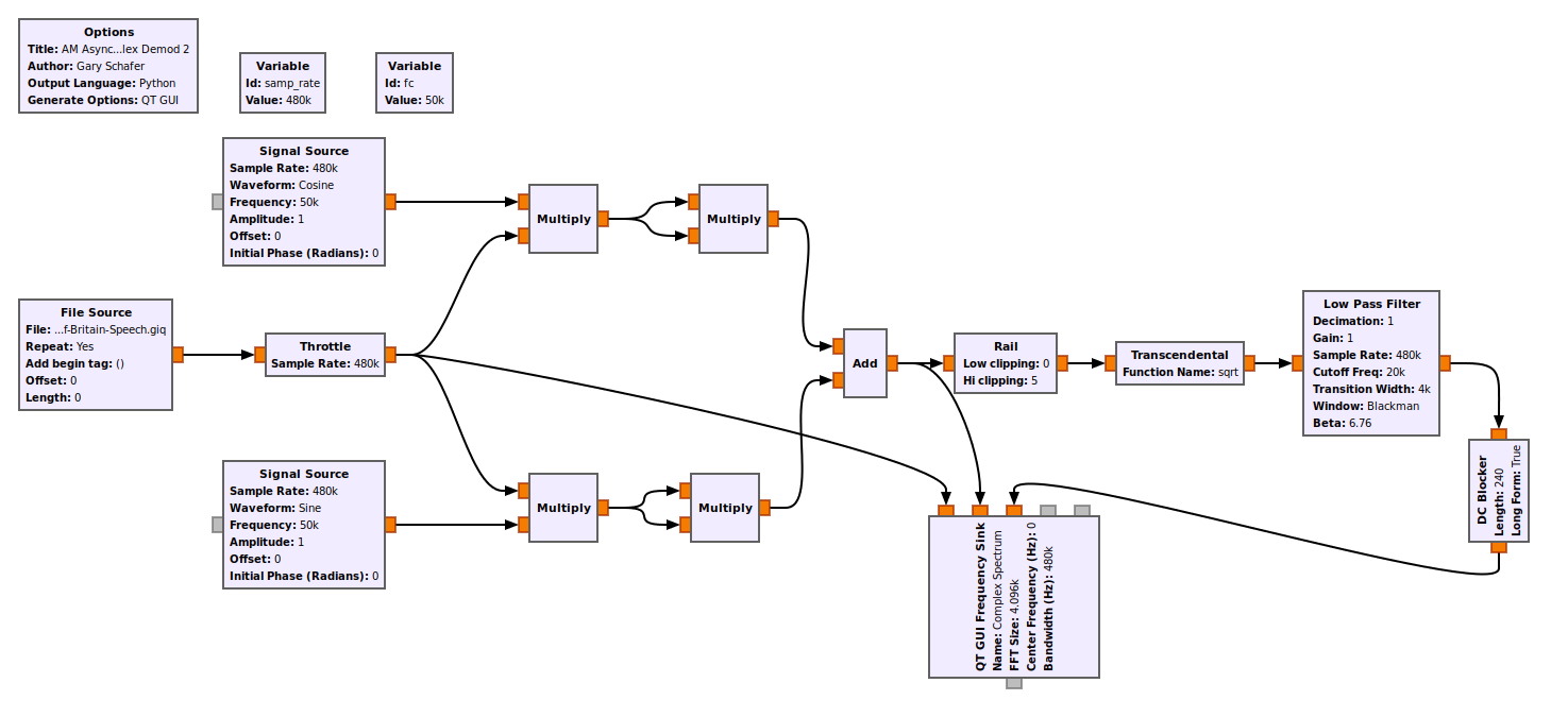
Graph to convert the incoming real signal into a complex signal using a quadrature demodulator. The two signal generators create a cosine and sine wave (sinusoids that are 90 degrees out of phase). These two signals are mixed with the real signal and converts it into a complex signal. Each leg (real and imaginary) is squared, added together, and lowpass filtered. All that's left is to perform the square root operation and remove the DC offset of the full carrier signal.
This is the spectrum of the of the original signal (black), the complex and squared signal (red), and the lowpass filtered signal (green).

According to Lyons's article:

This detector is asynchronous in operation because the local oscillators' fo frequency need not be equal to the fc frequency of the incoming modulated RF signal. An fo within 25% of fc is acceptable so long as the lowpass filters sufficiently attenuate spectral energy near |fc+fo| Hz.
Because the I(n) and Q(n) sequences are in quadrature, phase cancellation occurs in the adder such that only spectral energy in the vicinity of zero Hz appears at the adder's output. As such, this detector is very tolerant of local oscillator frequency/phase drift just so long as the local cosine/sine oscillators remain in quadrature.

However, what I discovered while playing around with this circuit was that the frequency of the sinewaves did not matter. The output signals looked the same regardless, and the signal properly demodulated regardless of the sinewave frequencies. I shifted it in 1 kHz increments between 0 - 100 kHz. The output was the same for all of them.

Synchronous Real Envelope Detection

This last one is the one that must be used if the AM signal is using suppressed carrier. Further, for some signals (digital, for example), the sinusoid generator must be in phase sync with the modulated waveform. However, if the signal is full carrier, then it becomes easier to deal with. A full carrier AM signal can be demodulated without having to phase sync with the modulated signal.

In the case of Gnu Radio, the input is probably already a complex signal. For example, if you are using any of the common, inexpensive SDRs (RTL-SDR, HackRF, SDRPlay, LimeSDR), then a full carrier AM signal could be demodulated simply by ensuring that the signal is properly filtered, followed by using a "Complex to Mag" block to recover the information.

For the case of a suppressed carrier AM signal, it depends on how tolerant the signal is to a frequency / phase offset. (NOTE: A frequency offset would create a constant phase offset, since frequency is a change of phase over time.) Audio signals, for example, could easily tolerate a frequency offset of tens of Hz. But a digital signal would require some type of frequency and phase synce. A friend of mine, an amateur radio enthusiast, states that a double sideband signal can be synced using a basic Costas loop. A single sideband, though? That would require a more sophisticated demodulator.

Unfortunately, the Costas loop in Gnu Radio is not the type that can be used on analog signals. It's designed for digital signals. Hence, I'll leave actual tests of coherent circuits for a later post (if I do one at all). UPDATE: The Costas loop can be used to demodulate suppressed carrier AM signals. It requires that the signal be double sideband, but otherwise the Costas loop will work using an "Order" of 2. The loop bandwidth almost always works fine with a value of "2*math.pi/100".

Summary

This was an interesting post to create. When I first started it, I figured it would take a few days to put it together. I've been working on it now for six weeks. Once again, Dr. Lyons piqued my curiosity enough that I've spent the past six weeks trying out different graphs in Gnu Radio, mostly for the noncoherent circuits.

Given what I've learned, I'd expect the squared circuit to be the best. Why? Because the spectrum only shows a signal at twice the original frequency. The other noncoherent circuits also have many harmonics. I consider those other harmonics to be wasted energy. They do not add anything to the demodulated signal. They're simply filtered out. The main thing I learned was that they all work for basic audio signals. Regardless of the graph, they all demodulate full carrier audio signals with little to no distortion. In my mind, the result is that I would choose the one that is the simplest to create in Gnu Radio.

Here's a Random Fact...