
Random Quote Board
Software Defined Radios and Spectral Displays
UPDATE: 4 January 2026: After attending a lecture by the renowned fred harris, I realized that a significant part of this post is, well, wrong. Specifically, the idea that "the FFT must operate on sample sizes that are a power-of-2". Prof harris explained how you can have a FFT that has sizes that are not a power-of-2. Not just that, but they can have almost any value. Some sizes will be faster than others, but you can have a truly "fast" Fourier transform for almost any size of FFT. Further, depending on the software and the hardware upon which it is operating, it's possible to have algorithms in which power-of-2 are slower than other sizes.
This post will cover digital spectral displays, with a focus on the spectral displays found on the most common software programs.
To start, we need to understand what a spectrum is. The term was coined by Sir Isaac Newton in a letter to the Royal Society in 1672 discussing how light was broken down into the rainbow of individual colors. Newton had used a prism in a beam of sunlight. Due to the frequency-dependence of refraction, the sunlight was broken down into its constituent colors.
Modern spectrum analyzers do the same thing, only with radio frequencies, not those at light frequencies. The most basic spectral display is a spectral trace. This is a power vs frequency display that (typically) shows power on the vertical axis and frequency on the horizontal axis. Think of this as a graph showing the correlation of a sinusoid at that frequency with the incoming signal.
What is Resolution Bandwidth?
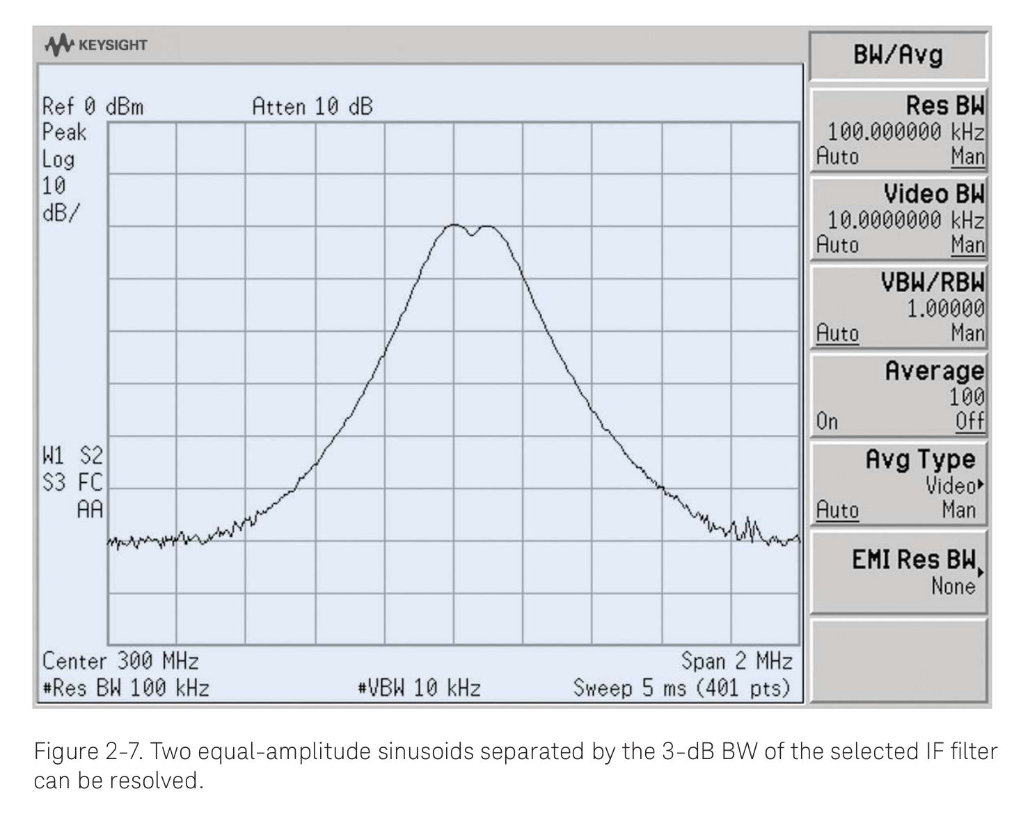
Resolution bandwidth is the ability of a spectrum analyzer to resolve (hence the name "resolution") two closely spaced signals. In the days of analog spectrum analyzers, this was measured with two equal amplitude tones (unmodulated sinewaves). You would get a display similar to that below:
Resolution bandwidth plays three, important roles in spectral analysis. These are:
- set the ability to resolve the fine spectral details of a signal: Resolution bandwidth is so called because of that first word, "resolution". As in "resolve". It was originally defined as the ability to resolve two, closely-spaced tones. I tend to think of it as the ability to see more detail on spectral data. A lower RBW means "more detail"; higher means "less detail".
- set the displayed noise floor: The combination of the RBW and the noise figure of the spectrum analyzer also sets the displayed average noise level (DANL). RBW and the noise level are directly related. You can see this below in the two spectra. The first, with a high RBW, also has a relatively high noise level. The second, with a lower RBW, also has a lower noise level. This is due to the basic fact that the spectrum analyzer will input a certain amount of noise. As the RBW goes down, that power is divided up into more and more bins. Each bin will receive a smaller share of the total power. The inverse is true. Increasing the RBW will also decrease the number of bins. Each bin will get a larger portion of noise.
- set the sweep time: The lower the resolution bandwidth, the more time required to cover a given span. Analog spectrum analyzers with a low resolution bandwidth require more time for narrower filters to settle (reach stability). Digital spectrum analyzers, including those from SDRs, require more samples in the time record in order to achieve a given low resolution bandwidth. Either way, you must have more time. There's no way around that.
With analog equipment, you had effectively an infinite number of points on your trace created by a noncoherent measurement of the signal power. The trace displays were smooth. They might look weird, but they were a smooth weird. If you want to know more about analog spectrum analyzers, I recommend the following:
- Keysight's "Spectrum Analysis Basics"
- Tektronix's "Fundamentals of Spectrum Analysis"
- Rohde and Schwarz's "Measuring with Modern Spectrum Analyzers"
- Anritsu's "Understanding Spectrum & Signal Analysis"
Let's talk about the differences between digital spectrum analyzers, and the analog ones that preceded them.
- Displays: Here's a quick overview of the differences in displays for spectrum analyzers.
- Analog: The first spectrum analyzers were all analog. As a matter of fact, they made use of analog oscilloscopes for the display, and simply added plugins to create the spectral information, both for the horizontal and vertical axes. The display itself would almost invariably be a cathode ray tube (CRT). This meant that the spectral information would be continuous.
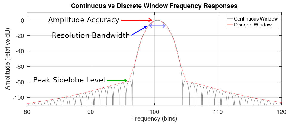
- Analog Data with Digital Display: Later spectrum analyzers, such as the Hewlett-Packard 8566 and 8568 spectrum analyzers, measured the signal levels using analog hardware, then digitized the amplitude information for display. The display itself might still be a CRT, but the information would be digital. This meant that the spectral information was now discrete, not continuous.
- Digital: The current systems, including software defined radios, only use analog components for the RF front ends. The RF front ends will use analog amplifiers, filters, oscillators and mixers. But shortly thereafter, the signals will be digitized and all of the spectral information will be calculated digitally, most likely using the fast Fourier transform (FFT), the speedy offspring of the discrete Fourier transform (DFT). The spectral information is discrete.
- Coherent vs noncoherent: Analog spectrum analyzers use noncoherent methods to measure the power at each frequency. The most common method for measuring amplitude is an actual amplitude demodulator, typically an envelope detector. Digital systems use the DFT. The DFT measures power at each point in a coherent manner. As fred harris stated in his paper, "The problem with this criterion is that it does not work for the coherent addition we find in the DFT. The DFT output points are the coherent addition of the spectral components weighted through the window at a given frequency."
- Spectral leakage: This is a problem specific to systems that create the spectral information digitally. Any system that uses the DFT / FFT will have this problem. Spectral leakage creates issues with the dynamic range in spectral analysis. The most-common solution, windowing, creates issues, too, including on the resolution bandwidth.
For understanding the digital version (DFT / FFT), I strongly recommend either Richard Lyon's "Understanding Digital Signal Processing" or Steven Smith's "The Scientist and Engineer's Guide to Digital Signal Processing". Actually, for these two, get both.
Resolution Bandwidth: How It Is Measured
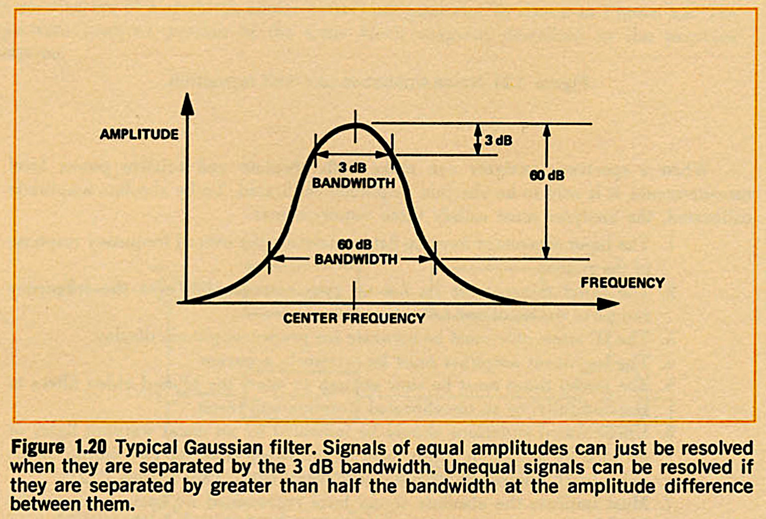
A key issue of resolution bandwidth is understanding how it is measured. In analog spectrum analyzers, its measured at points 3 dB down from the peak of the (typically Gaussian) filter. Further, analog filters also have a parameter known as the selectivity. This refers to how quickly the filter goes from little to no attenuation to a lot of attenuation. It's typically measured as a ratio between the bandwidth at the 3 dB points (again, which is the RBW), and at points 60 dB down from the peak.
The DFT is different. As we go into more detail about digital spectra, we'll build up to an understanding of resolution bandwidth with respect to the DFT.
The Discrete Fourier Transform and Binwidth
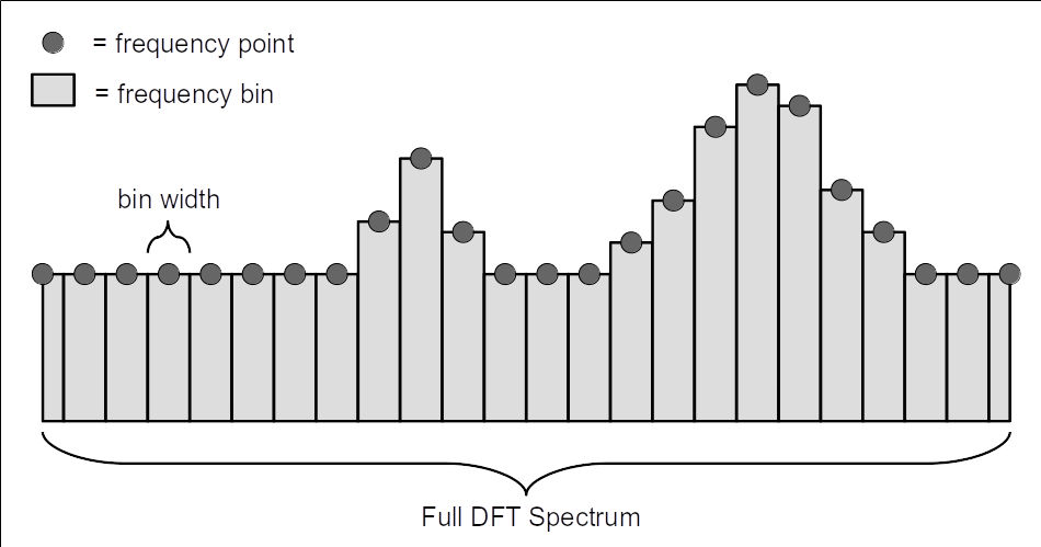
The discrete Fourier transform (DFT) creates a discrete spectrum consisting of a series of points. Each point represents a bin, meaning a certain amount of spectrum. The bandwidth of each bin is a binwidth. The binwidth can be calculated as follows:
Binwidth = fs/N
where:
- fs = sample rate
- N = length of time record, in samples
The Discrete Fourier Transform and Windowing
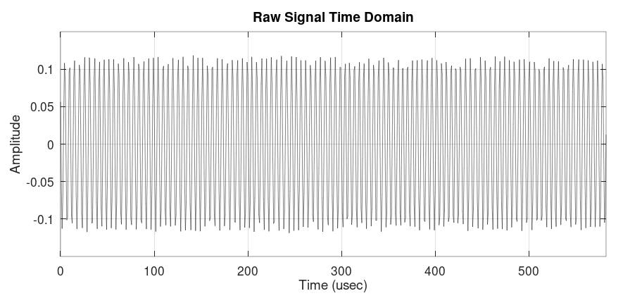
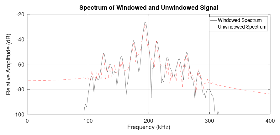
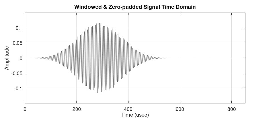
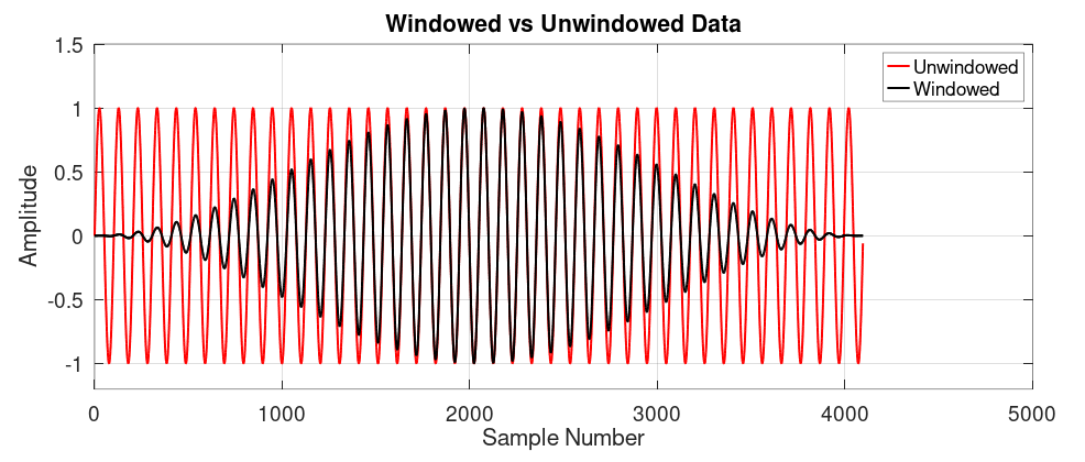
Let's say that we have a time record of a signal. Further, let's say that we take this time record and plug it directly into the DFT algorithm. Here's how the corresponding time domain and frequency domain displays would appear.
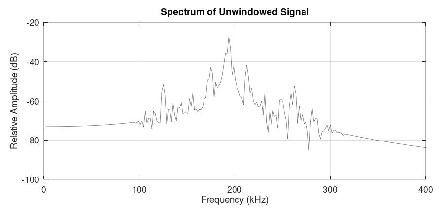
Spectral leakage, which honestly sounds like a really bad medical condition that I might have as I pass through middle age, creates problems in the spectrum. This includes scalloping loss (an improper amplitude level) and poor dynamic range. It is not something that has an equivalent in the analog world; it is strictly a problem of the digital spectrum. To alleviate these problems, a digital window is applied. A window is a set of weights applied to each point of the time record such that the ends are pushed to zero, or close to it.

Windowing and Resolution Bandwidth
Windowing has several effects on the spectral trace. This includes the resolution bandwidth, the dynamic range, and amplitude accuracy.
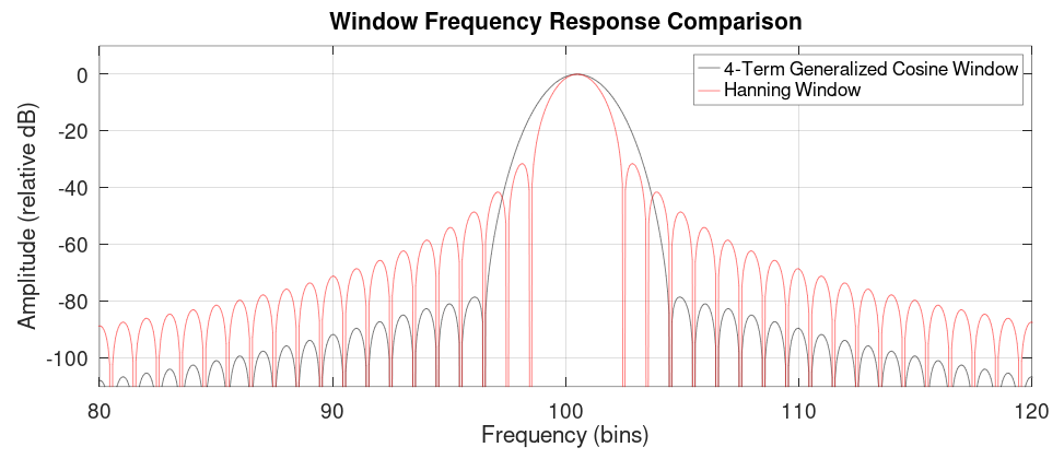
There are a host of different windows possible. A good overview as well as analysis of different windows is fred harris' "On the Use of Windows for Harmonic Analysis with the Discrete Fourier Transform".
This is where we point out the difference between analog and digital resolution bandwidth. As fred harris pointed out (with my emphasis added):
The classic criterion for this resolution is the width of the window at the half-power points (the 3.0-dB bandwidth). This criterion reflects the fact that two equal strength main lobes separated in frequency by less than their 3.0-dB bandwidths will exhibit a single spectral peak and will not be resolved as two distinct lines. The problem with this criterion is that it does not work for the coherent addition we find in the DFT. The DFT output points are the coherent addition of the spectral components weighted through the window at a given frequency.
If two kernels are contributing to the coherent summation, the sum at the crossover point (nominally half-way between them) must be smaller than the individual peaks if the two peaks are to be resolved. Thus at the crossover points of the kernels, the gain from each kemel must be less than 0.5, or the crossover points must occur beyond the 6.0-dB points of the windows...it is the 6.0-dB bandwidth which defines the resolution of the windowed DFT."On the Use of Windows for Harmonic Analysis with the Discrete Fourier Transform", fredric harris, Proceedings of the IEEE, Vol. 66, No. 1, January 1978
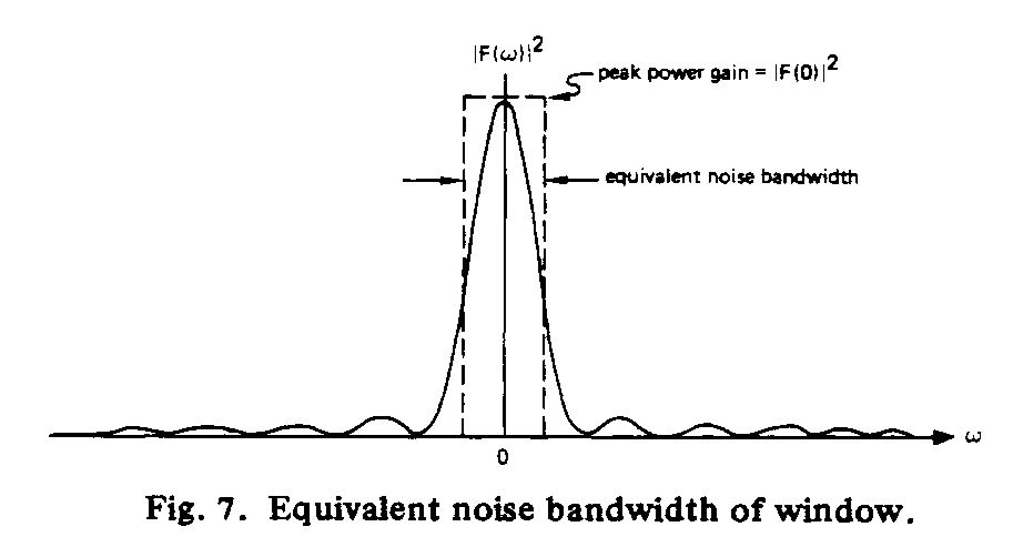
Using the 6 dB point is not widely accepted. Instead, most systems use the normalized equivalent noise bandwidth (NENBW). The equivalent noise bandwidth (ENBW) is the bandwidth of an ideal, brickwall filter that passes the same amount of power as does the window spectrum. The normalized ENBW is an ENBW that has been scaled by the number of samples used to create the window. The NENBW does not have a point measurement such as with the 3 dB, 6 dB or 60 dB points on a filter spectrum. Instead, it must be calculated from the values of the window weights (discussed below) placed on the time record before it is input to the DFT.
Quick digression: I attended an online presentation by professor harris in 2024. During the Q&A afterwards, I asked why the industry went with the NENBW for measuring resolution bandwidth rather than the 6 dB that would have made the measurements more backwards compatible with analog systems. He said it was due to the simplicity. "The equivalent noise bandwidth is easier to measure," is what he said precisely. You can quickly calculate the window factor value from the window weights, whereas with the 3 dB or 6 dB points, its more complicated (and more processor intensive).
Thinking about it, using the ENBW as your RBW means that you can quickly calculate the noise power spectral density from a basic spectral power measurement. Simply divide the measured power by the RBW, and you have the
- Simplicity: It's straightforward to calculate the NENBW once you've calculated the window weight values. The amount of processing is relatively minimal, even for systems performing real-time measurements. This makes it advantageous, especially for the early systems in which processing power was not nearly as high as it is now.
- Measuring Noise PSD: If you use a spectrum analyzer that measures spectral power weighted with a window whose NENBW we know, then we can calculate the noise spectral density by simply dividing the measured power by the ENBW.
With the addition of windowing, the calculation for the resolution bandwidth is as follows:
RBW = β * fS / N = β * binwidth
where:
- β = window bandwidth factor, a value that depends on the window used and the parameter of the selected window desired. As stated in the harris' paper, "The coefficient β is usually selected to be the ENBW in bins...". That's also called the "normalized equivalent noise bandwidth" or "NENBW".
- fS = sample rate
- N = length of data samples in the time record
According to harris, the NENBW can be calculated as:
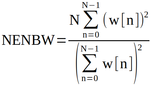
Where:
N = number of data samples in time record
w[n] = values for window
The table below lists some common windows and their respective 3 dB, NENBW, and 6 dB window bandwidth factors.
| Window | β Value | ||
|---|---|---|---|
| 3 dB BW | NENBW | 6 dB BW | |
| Uniform | 0.88589 | 1.000000 | 1.206713 |
| Hanning | 1.44058 | 1.500000 | 2.000000 |
| Hamming | 1.302985 | 1.362826 | 1.81523 |
| Blackman (approx) | 1.643684 | 1.726757 | 2.298803 |
| 4-Term Minimum Blackman-harris | 1.899448 | 2.004353 | 2.666428 |
| Nuttall (used in Spike) | 1.915462 | 2.021233 | 2.688750 |
| Stanford Research Flattop ("Flattop" in Spike) | 3.731197 | 3.770164 | 4.592665 |
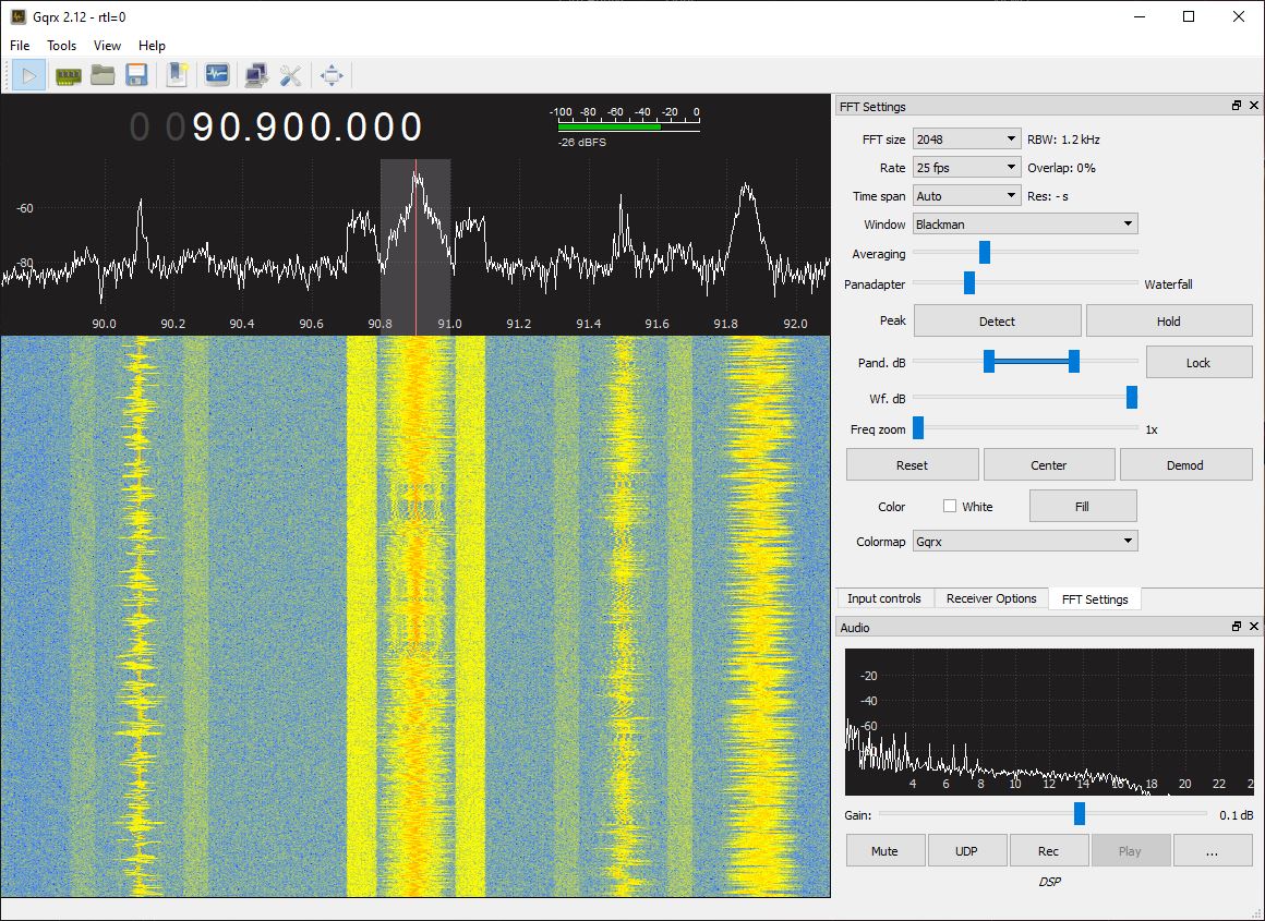
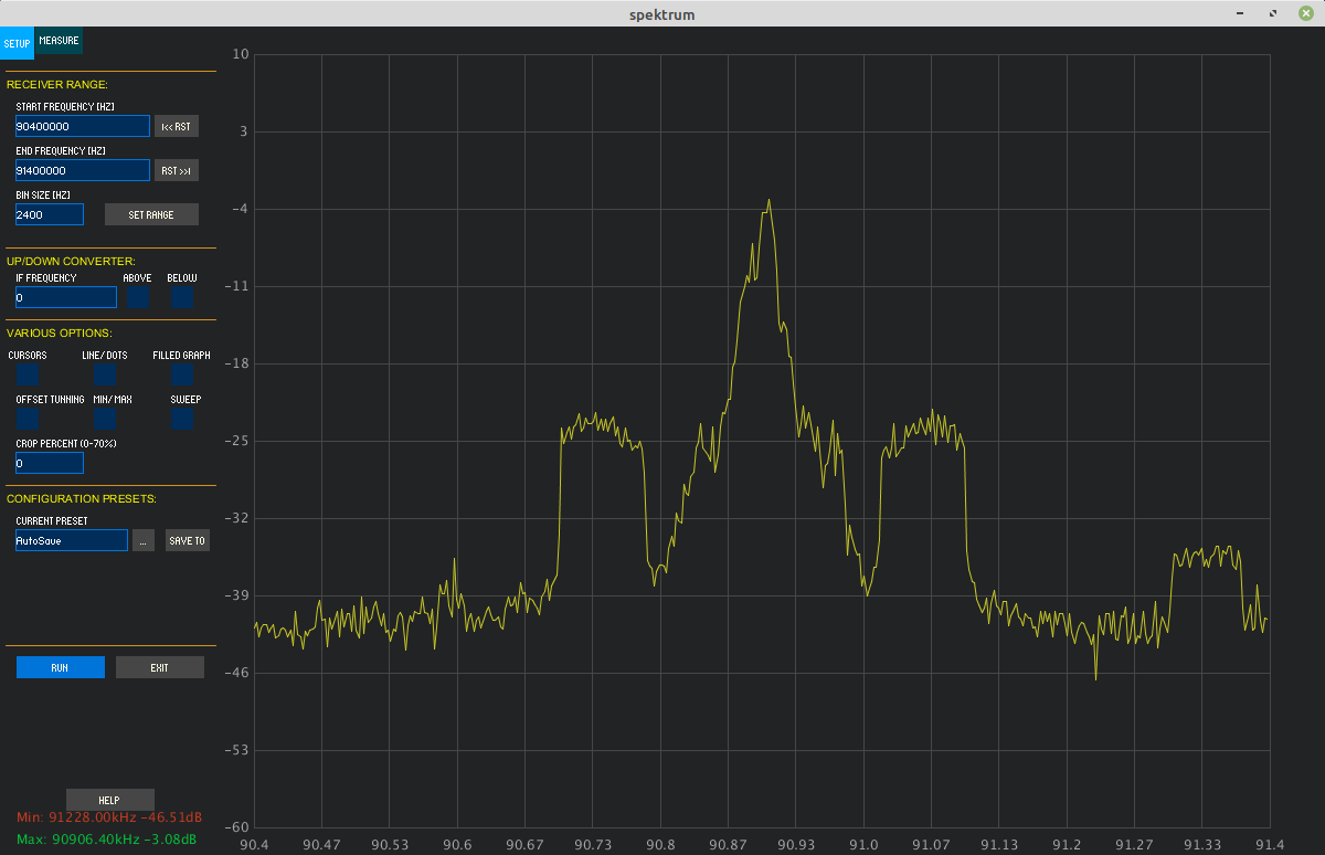
For example, using a Blackman window (NENBW = 1.726757), a 2.4 MHz sample rate, and a 2048 point DFT, the resulting RBW = (1.726757)(10e6)/(2048) = 2023.6 Hz. These are the settings and the RBW for the GQRX display shown below.
The FFT and Zeropadding
Up til now, we've talked about the discrete Fourier transform or DFT. The idea of calculating the spectral values digitally (e.g. with a computer) didn't really take off until Cooley and Tukey published their paper explaining how to perform the DFT in an extremely efficient manner. This is now what we call the fast Fourier transform or FFT. Since then, several other "divide-and-conquer" algorithms have been developed. This includes the variants of the Cooley-Tukey, Good-Thomas, Rader, and Winograd. These various algorithms operate on different numbers of sample sizes. All of the most popular software routines, however, appear to use algorithms that require the length of the time record to be a power-of-2.
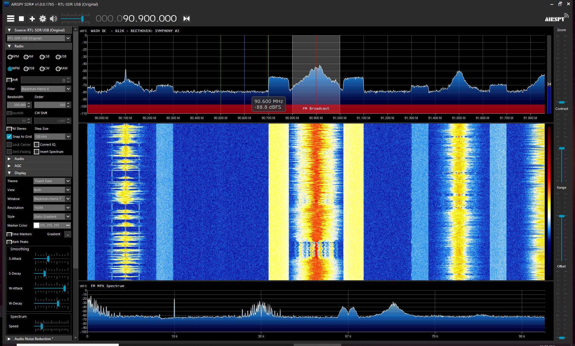
For example, the GQRX display is 2048 points (211), while the Airspy display is 16384 samples (214).
Here's the problem. If the sample rate is fixed, then the available resolution bandwidths will be limited by the fact that the time record must be a power-of-2. If we adjust the number of samples in the time record (N), then it may not be a power-of-2. This is where zeropadding comes into play. We can literally add samples consisting of 0s to the end of the time record until the number of samples is a power-of-2. For example, look at the 700 point time record. By adding 324 0s to its end, we create a 1024 (210) time record.
The original, unmodified DFT requires N2 operations, while a full FFT only requires N*log2N. To give you an idea of the savings in computations by zeropadding, take a 1741 point time record. The number 1741 is a prime number. It cannot be factored. It would require the full N2, or 3031081, computations to calculate the DFT. But what if we added 307 zeros to the record? It would now be 1741 + 307 = 2048. This is a power-of-2. It would only require N*log2N = 2048*11 = 22528 computations. Despite the fact that the time record is larger, it would require less than 1/100th of the amount of calculations. It would also have the benefit of slightly reducing any amplitude inaccuracies.
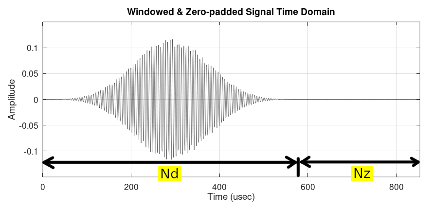
Looking at the zeropadded time record, it consists of two segments.
- data samples: this has a length of Nd. The data samples are the only ones that matter for calculating the resolution bandwidth.
- zeros: this has a length of Nz. These do not matter for calculating the resolution bandwidth. They are used to interpolate the spectrum and/or create a time-record length that is a power-of-2.
The total length of the time record is: N = Nd + Nz.
NOTE: If employing zeropadding, the time record should be windowed first, then zero padded.
There are two things about zeropadding and the spectral display. These are:
- The resolution bandwidth only depends on the length of the data segment (Nd): If the time record was not zero padded, its length would be the Fourier transform convolved with the rectangular impulse. By adding zeros, there's no new information being added, which means that the resolution bandwidth will not change.
- The binwidth depends on the total length of the time record (N = Nd + Nz): Zeropadding does not add any new information, but it will lower the binwidth. The result of this on real world signals is that, as more zeros are added, the DFT becomes closer to being the discrete time Fourier transform (DTFT), meaning that the time domain is discrete, but the spectrum is continuous.
The Variable RBW
Signal Hound's Spike software is different from most other software for SDRs. It allows the user to create a user-provided resolution bandwidth. How does it do this? Remember how the RBW is calculated for a DFT:
RBW = β fS / Nd
where:
- β = window bandwidth factor, and typically the NENBW of the window.
- fS = the sample rate used to create the digital time record
- Nd = the length of the data segment of the time record.
Given a particular window, there are two variables that can be adjusted to create a variable bandwidth spectral display. These are the sample rate and the length of the data segment. It's typically easier to keep the sample rate fixed, and adjust the number of samples collected into the data segment of the time record. This is precisely what Spike does.
Spike takes the user-provided resolution bandwidth, a fixed sample rate[1], the chosen window (Nuttall or flattop for the BB60C), and calculates the number of samples needed in the data segment. It zero pads the rest of the time record to make it a power-of-2, then calculates the FFT of the time record.
The calculation for the required number of data samples can be found by re-arranging the equation above.
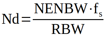
Where:
Nd = number of data samples in time record
NENBW = normalized equivalent noise bandwidth
fs = sample rate of Signal Hound device (= 40 MHz for BB60C)
RBW = desired resolution bandwidth
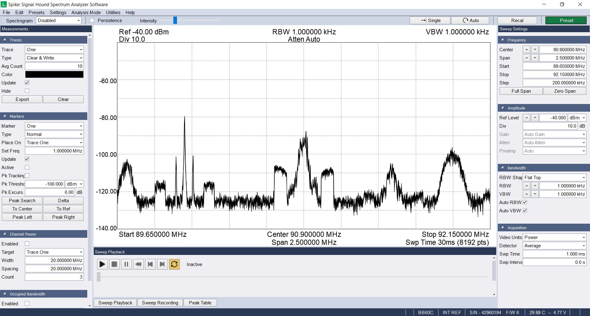
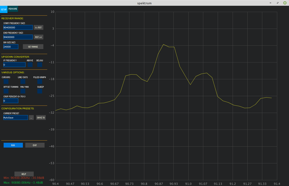
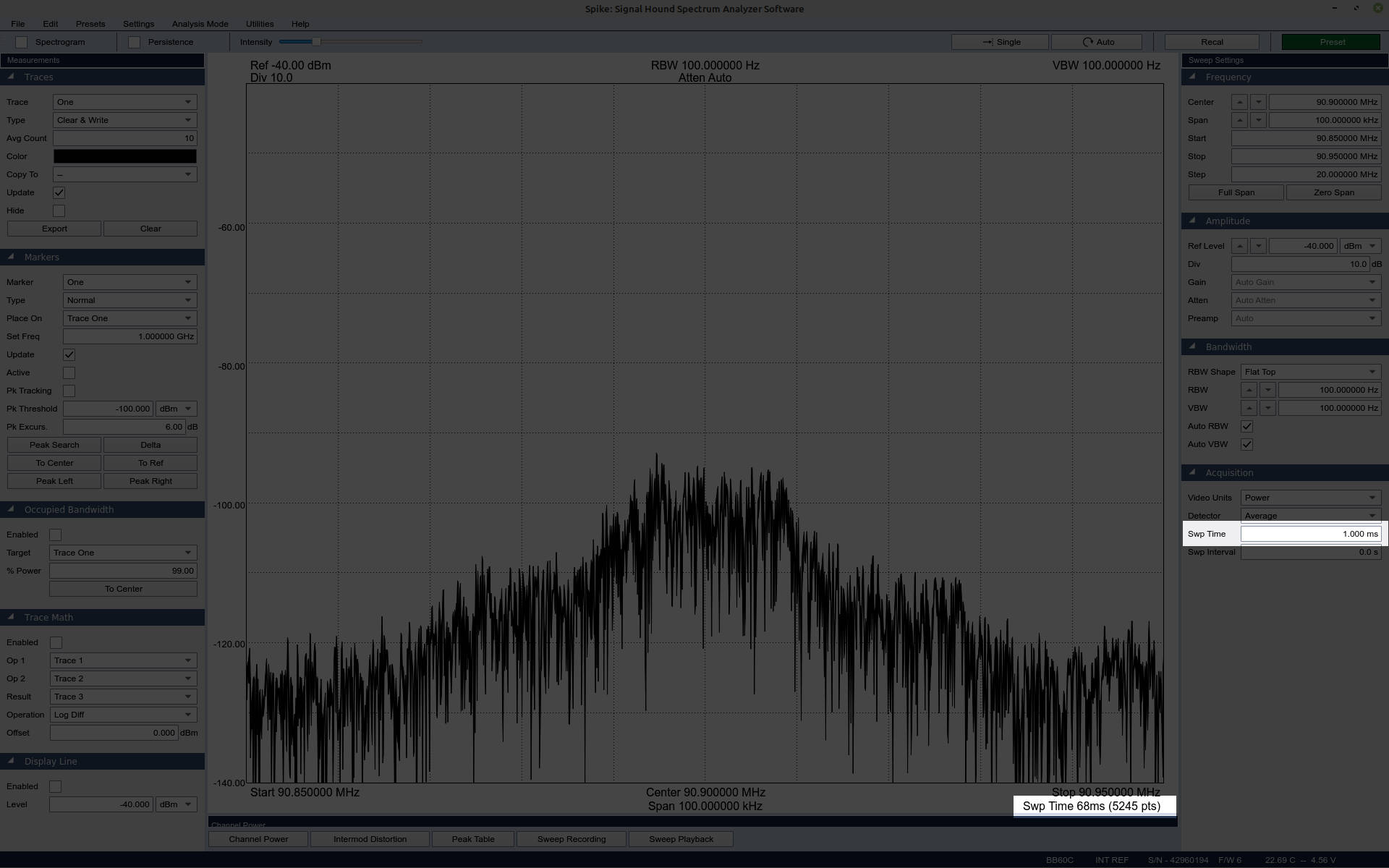
Take the following example showing the FM broadcast band using the user-provided resolution bandwidth of 30.33 kHz using a Nuttall window. This particular Nuttall window has a NENBW = 2.0212.
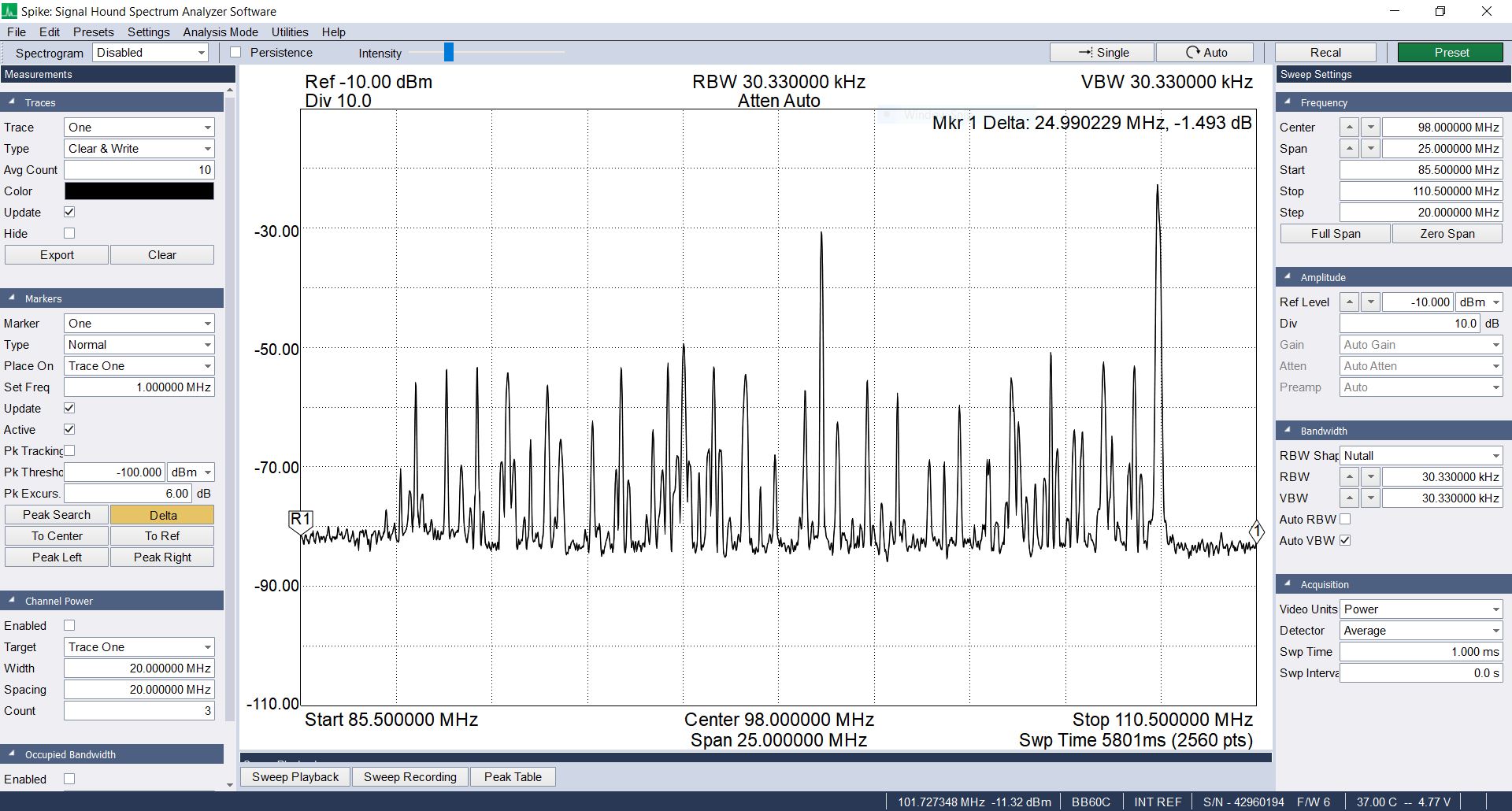
Since we're talking about the Spike software, there's one other aspect of the spectral display. With the fixed sample rate (40 MHz) and the length of the time record (4096 points once zero padded), this means that the binwidth is (40e6)/(4096) = 9765.6 Hz. Given the set span of 25 MHz, this requires a total of (25e6)/(9765.6 Hz) = 2560 points. Note that that is the length of the sweep, shown in the lower, righthand corner just underneath the "Stop" frequency of the display.
The Detector
As if this wasn't complicated enough, there are a couple of other parameters with respect to spectral displays. When spectrum analyzers began switching from analog to digital displays in the mid 1970s, they discovered a problem. Analog displays, because they were continuous in frequency, showed every, possible spectral point. Digital displays were different. Digital displays are similar to the screen on which you're reading this. They have a finite resolution. Engineers had to figure out how to display an infinite number of points on a finite display. The local oscillator (LO) tuner steps at some fraction of the resolution bandwidth. The RBW, in turn, is a fraction of the overall span. This means that a display may have thousands of points of spectral data, but only hundreds of actual display points. Some mechanism must be used to reduce the spectral points to the available display points. This led to the use of detectors. There are a myriad of different detector types, but their purpose is the same. A detector reduces the number of spectral points collected to those that can be displayed on the available screen size.
Digital systems add an additional parameter, time. The reason for this harks back to the concept of windowing (discussed above). While windowing reduces issues related to spectral leakage (poor dynamic range, scalloping loss), it also reduces the amount of signal available to process.
To deal with this problem, some systems now use overlapping windows. This means the system collects a time record, then subdivides the time record into a series of overlapping, windowed time records.
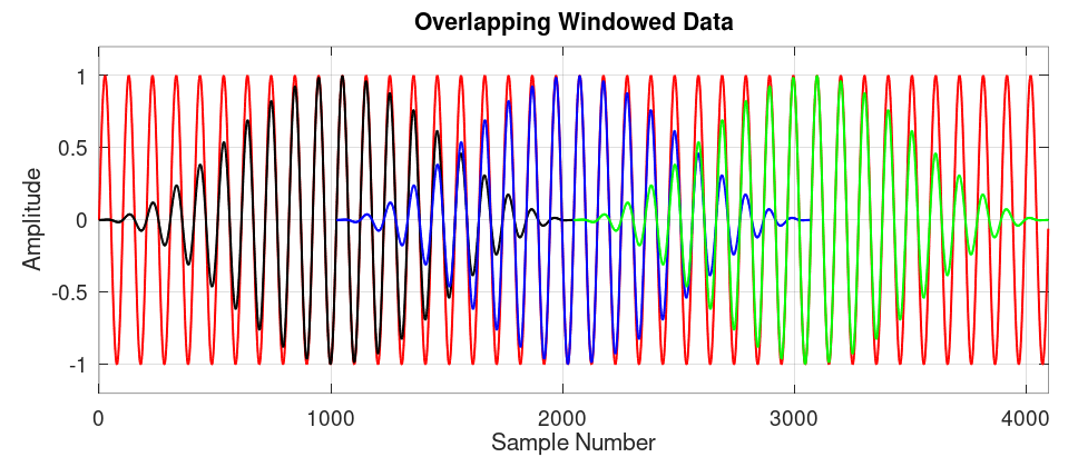
Most, basic SDRs do not provide overlapping windows to create spectral displays. Signal Hound's Spike is no ordinary SDR software. It's default is to collect a certain time, subdivide the collected time record into a series of overlapping windowed time records (with the length of each windowed time record determined by the resolution bandwidth), zeropad each record such that it is a length that is a power-of-2, calculate the FFT of each record, then use the detector to calculate the actual displayed value.
The amount of time with which Spike collects data is listed on the right of the screen as "Swp Time". The default value is 1 msec. Spike will attempt to collect 1 msec of data for each step of the tuner. With its 40 MHz sampling rate, its collecting (40e6)(1e-3) = 40,000 samples for each step. Given that most resolution bandwidths only require a few hundred to a few thousand samples per time record, this provides the ability for Spike to create many overlapping windowed time records.
Take, for example, a spectral trace with 100 kHz RBW and the Nutall window. The number of data points would be:
Nd = (40e6)(2.01212)/(100e3) = 808.48 ≈ 808 points
The amount of time that the digitizer is actively collecting data samples is called the acquisition time. The FFT will need 808 samples to provide the requested 100 kHz RBW. The first 808 samples will come from the beginning of the acquired 40,000 sample time record. After that, the samples chosen for each subdivision is determined by the amount of overlap. The amount of overlap is determined by the window chosen. Windows that suppress more of the signal require greater overlap to compensate for it. For the particular Nuttall window used, the optimum amount of overlap will be roughly 66%. This equates to roughly (2/3)(808) = 539. This means that the second data set will use 539 samples from the first data set, and only 808 - 539 = 269 new samples. It will continue this until all 40000 samples have been used. This will allow for roughly (40000)/269 ≈ 149 FFT records. This, in turn, means that each frequency point will be represented by 149 different samples.
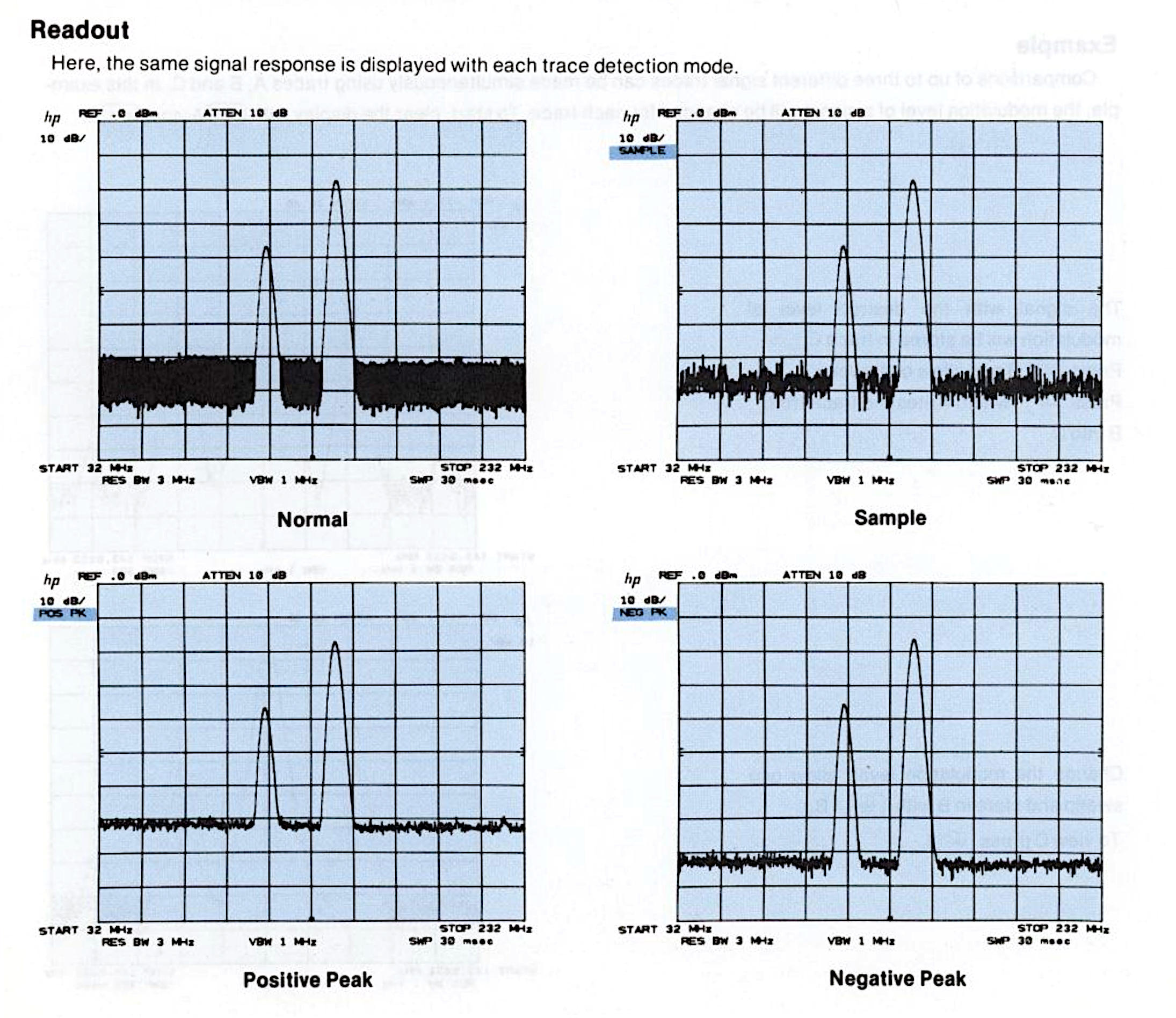
Which leads back to the detector. Spike provides four detectors with which we can choose from this dataset. These are sample, minimum, maximum, and average. Spike also allows for the display of something called "min/max". In this case, probably every displayed odd sample is the "max" value, while every displayed even sample is the "min" value.
All of this, the acquisition time, plus the time required to calculate all of the FFTs and display the final result, called the processing time, leads to the measured sweep time. That's the value displayed below the spectral trace.
The Binwidth and Span
The last part is to pull out the number of frequency points needed for the desired span. Digital displays use discrete frequency points. The span must be an integer number of frequency points. This means that arbitrary spans are not possible. It can only be within 1/2 of a binwidth.
Summary of Steps to Create Digital Spectral Display
This is the flow of a basic spectral display. This does not take into account zeropadding, overlapping windows, or detection.
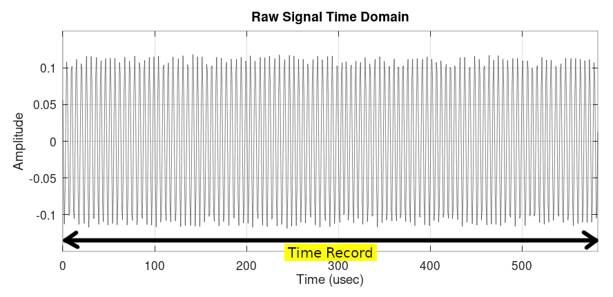
Step #1) Collect the data samples into a time record. These are the data samples that will ultimately be fed into the fast Fourier transform (FFT). This particular time record consists of 700 samples.
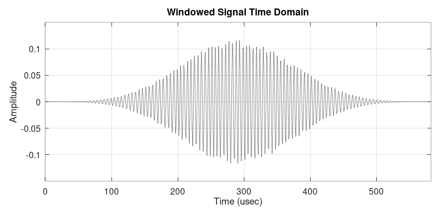
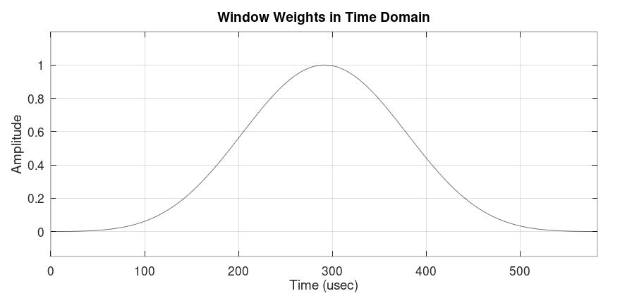
Step #2) Window the data. This is how the windowed time record appears. Again, the window does nothing more than weight the amplitudes of the samples in the time record. By having the ends approach or be set to zero, this alleviates much of the scalloping loss and spectral leakage when the time record is fed into the DFT algorithm.
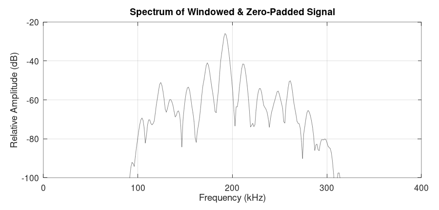
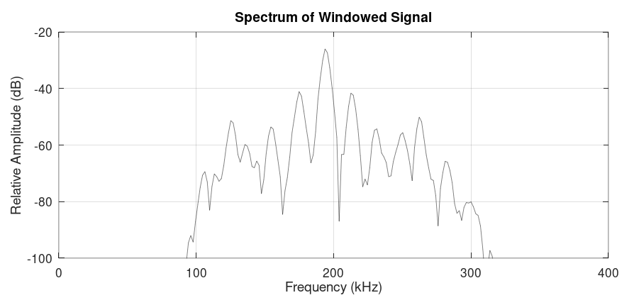
Step #3) Calculate the FFT of the windowed time record. This is the spectrum of the windowed time record after it has been passed through the FFT. The last part of this step is to calculate the power of each spectral point to make it either a "dB" or (if calibrated) "dBm".
Resolution Bandwidth As Stated in Various Programs
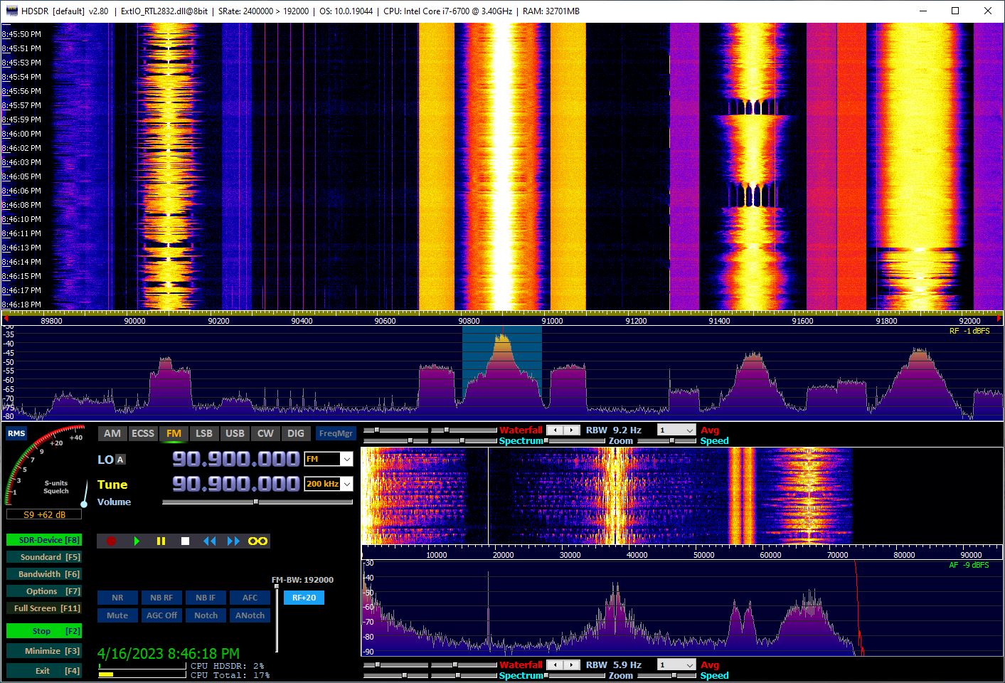
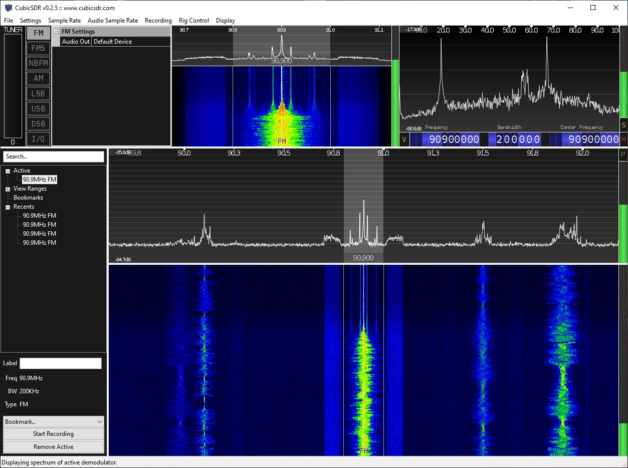
I've played around with many, different software defined radios. This includes the already-mentioned Signal Hound BB60C, the Great Scott Gadget's HackRF One, several, different RTL-SDRs, the LimeSDR Mini, and a SDRplay RSP1A. All are controlled from software, whether it's GQRX, Gnu Radio Companion, Airspy's SDR#, HDSDR, or CubicSDR. All of the SDRs provide complex samples to this software, and the software performs the calculations that create the spectral displays. All of these programs provide spectral displays. Most do not provide resolution bandwidth (RBW) values, despite the fact that they do have measurable resolution bandwidths.
CORRECTION: Based on a misreading (my bad) of the Signal Hound BB60C Manual, I first stated that the sample rate of the BB60C was 40 MHz, then I corrected that to 80 MHz. So, which is it? It's 40 MHz. How do I know that? Two places. First, here's the problematic statement in the BB60C manual (my emphasis added):
From the ADC, digitized IF data is handed off to an FPGA where it is packetized. The Cypress FX3 peripheral controller streams the packetized data over a USB 3.0 link to the PC, where 80 million, 14-bit ADC samples per second are processed into a spectrum sweep or I/Q data stream.
The key is "processed into a spectrum sweep or I/Q data stream." In other words, it's 80 million samples, but they've not been turned into IQ samples as that term is understood. An IQ sample is actually two samples, an I (in-phase) and Q (quadrature), that, together, are considered one "IQ sample".
This leads to the second way I know that the sample rate is actually 40 MHz. The Signal Hound BB60 API shows a table for the "bbConfigureIQ" statement. The first line of the table shows "Sample Rate (IQ pairs/s)" of "40 MS/s" (40 millions samples per second), and a decimation rate of "1". This is thus the sample rate of the system.
Sigh. I've corrected the post. Again. Hopefully for the last time.