Understanding SSB with Gnu Radio

Gary Schafer, August 2025

I've been helping Paul Maine "The SDR Guy" to understand how to use Gnu Radio for single sideband (SSB) demodulation using analog techniques. This helped me, too, to understand how the various analog methods of SSB demodulation and modulation work. I'm going to document what I learned here.

NOTE: Most of the Gnu Radio flowgraphs shown here are for the purposes of explaining and understanding analog techniques. They are not designed for efficiency in a digital signal processing (DSP) system; they are designed to educate.

But, ya know, they do work...

SSB Review

If you're looking for a general review of the different "flavors" of AM, take a look at my post on AM demodulation using digital signal processing techniques.

SSB has been around for just over 100 years. John R. Carson in 1915 invented a SSB method as a way to pack in more telephone calls on long distance circuits¹. SSB is a form of amplitude modulation (AM). I say that because, as I was reviewing my notes on SSB, I found a lot of tech writers who talk about "SSB" and then they talk about "AM". The reason is that, according to them, "SSB" refers to a specific form of amplitude modulation in which you're only transmitting a single sideband (as opposed to both sidebands) without the reference signal that everyone calls the "carrier" (a term I dislike, but I have to respect history). In abbreviated form, this is AM-SSB-SC. You can also explain it as the specific sideband being transmitted, such as AM-LSB-SC (lower sideband) or AM-USB-LC (upper sideband). "AM", on the other hand, refers to a double sideband and full carrier, or AM-DSB-FC.

There are three analog methods for generating SSB signals. These are filtering, phasing, and Weaver. Let's review each of them.

SSB Modulation with Filtering

To me, this is the most straightforward method for making single sideband (SSB). Create a double sideband (DSB) signal, then filter out the undesired sideband.

Block diagram showing an audio source passing through a mixer, which is also fed by a local oscillator. The output of the mixer passes through a bandpass filter to create a single sideband modulated signal. — Block diagram showing how the filtering method works. The audio signal is modulated as a double sideband (DSB) AM signal, then the undesired sideband is filtered out using the bandpass filter (BPF).

Gnu Radio flowgraph block diagram showing blocks starting with an audio source, passing through a throttle block, through a rational resampler block, then into a multiply block. A signal source captioned as a local oscillator feeds the second input of the multiply block. The multiply block is also captioned as a mixer. The output of the multiply block feeds into a bandpass filter, which is captioned as the filter that removes the upper sideband and leaves the lower sideband. The output of the bandpass filter feeds into a frequency sink acting as a spectral display. — Gnu Radio flowgraph to create a basic single sideband (SSB) modulated audio signal. The audio source is multiplied by a signal source, which is the local oscillator. The "Multiply" block is the mixer. The output is the double sideband signal. The bandpass filter only passes the lower sideband, removing the upper sideband. The output is the complete SSB signal, which is LSB in this instance.

Display of two spectral displays, one over the other. The top one shows a signal at 0 Hz, the baseband signal, followed by another signal at 60 kHz, which is a double sideband AM signal. The bottom display shows the 60 kHz signal after it has passed through the bandpass filter. Only the lower sideband remains. — Spectral displays of the audio signal as it first appears coming out of the audio source (top display, left in black) and after it has been modulated as a double sideband signal (top display, red at right). The bandpass filter removes the upper sideband, leaving only the lower sideband, single sideband signal (bottom display).

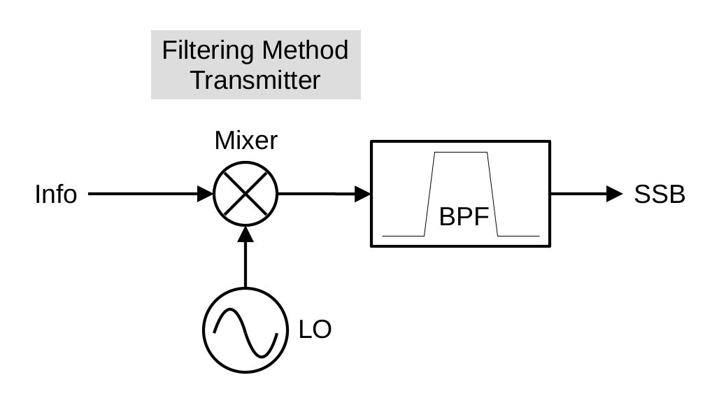
That's pretty much it. According to Miller's and Beasley's "Modern Electronic Communication (Seventh Edition)"², the filter method predominated because (a) it was the simpler method and (b) it worked well enough to suit most people's purposes. Essentially (according to them), the phasing and Weaver methods might have provided better removal of the undesired sideband, but (as you'll see) they're also more complicated.

However, according to McElroy:

By April of 1950, the magazine [Refers to QST magazine - Gary] would report that hams using phasing methods outnumbered those using filter 2 to 1.

I'll let you decide which one was more popular. Let's continue on.

SSB Modulation with Phasing

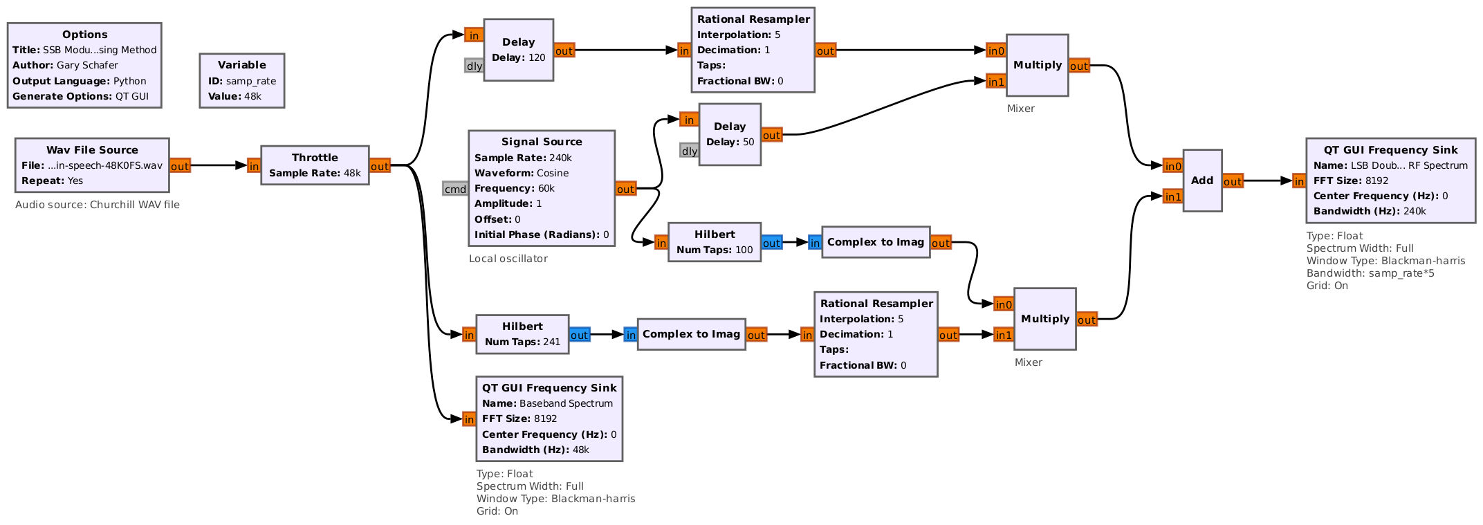
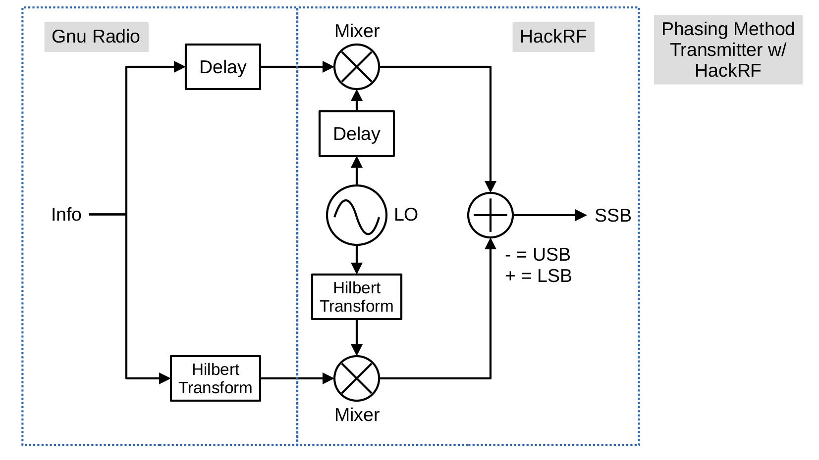
The phasing method is actually very similar to the filtering method. The only difference is that it filters out the lower sideband before modulating it onto the RF carrier. Let's start with the block diagram of the phasing method.

Block diagram showing the word info radiating two arrows, one going up and the other down. The arrow going up connects into a block marked delay. The arrow going down connects into a block marked Hilbert transform. In the center ranked vertically are, starting at the top, a circular blocked marked mixer, followed by a block marked delay, another circular block marked LO, a block marked Hilbert transform, and another circular block marked mixer. Arrows come out of the LO block and go up and down. Both end in the mixer blocks after passing through the delay (upper) and Hilbert transform (lower) blocks. The delay block from the info on the left connects into the upper mixer, while the Hilbert transform from the info connects into the lower mixer. The outputs of both mixers connect to a circular block on the right with a plus sign in the center and marked add. To the right of this add block are the words plus equals LSB and minus equals USB. An arrow comes out of the add block with the caption SSB. — Block diagram of a phasing method modulator. The information (audio, typically) is split, with one going to a delay block (upper) and the other going to a Hilbert transform (lower). The purpose of the delay block is to ensure that the signals passing through both upper and lower branches align at the end. The Hilbert transform takes the input signal and shifts its phase by -90 degrees. One way to think of this is that, if the input is a cosine, the output of the Hilbert transform will be a sine. The upper branch can now be considered the in-phase (I) branch, while the lower branch is the quadrature (Q) branch. The local oscillator (LO) passes through a delay for the upper branch and a Hilbert transform for the lower branch. This effectively makes it a complex sinusoid. The I branch is mixed with a cosine (effectively) while the Q branch is mixed with a sine. The outputs of the mixers can be added or subtracted to create the final SSB signal. Adding creates a LSB signal, while subtracting them creates the USB signal.

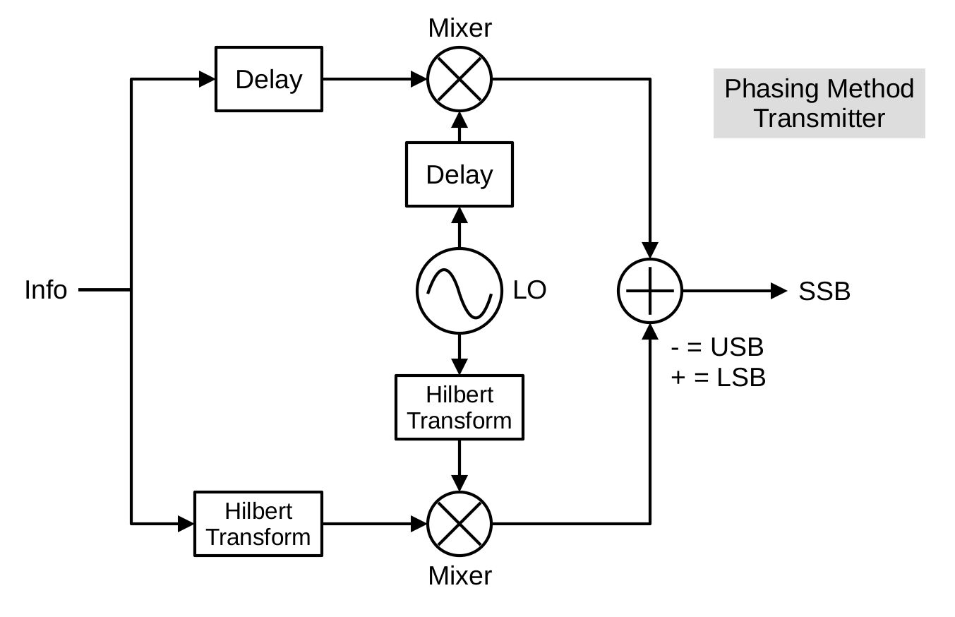
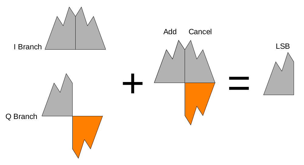
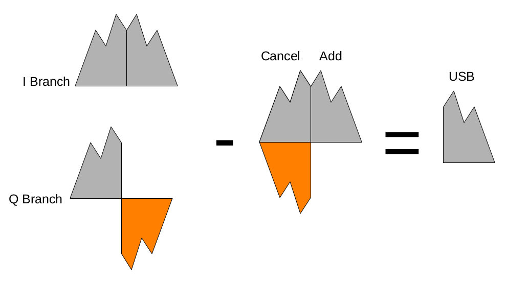
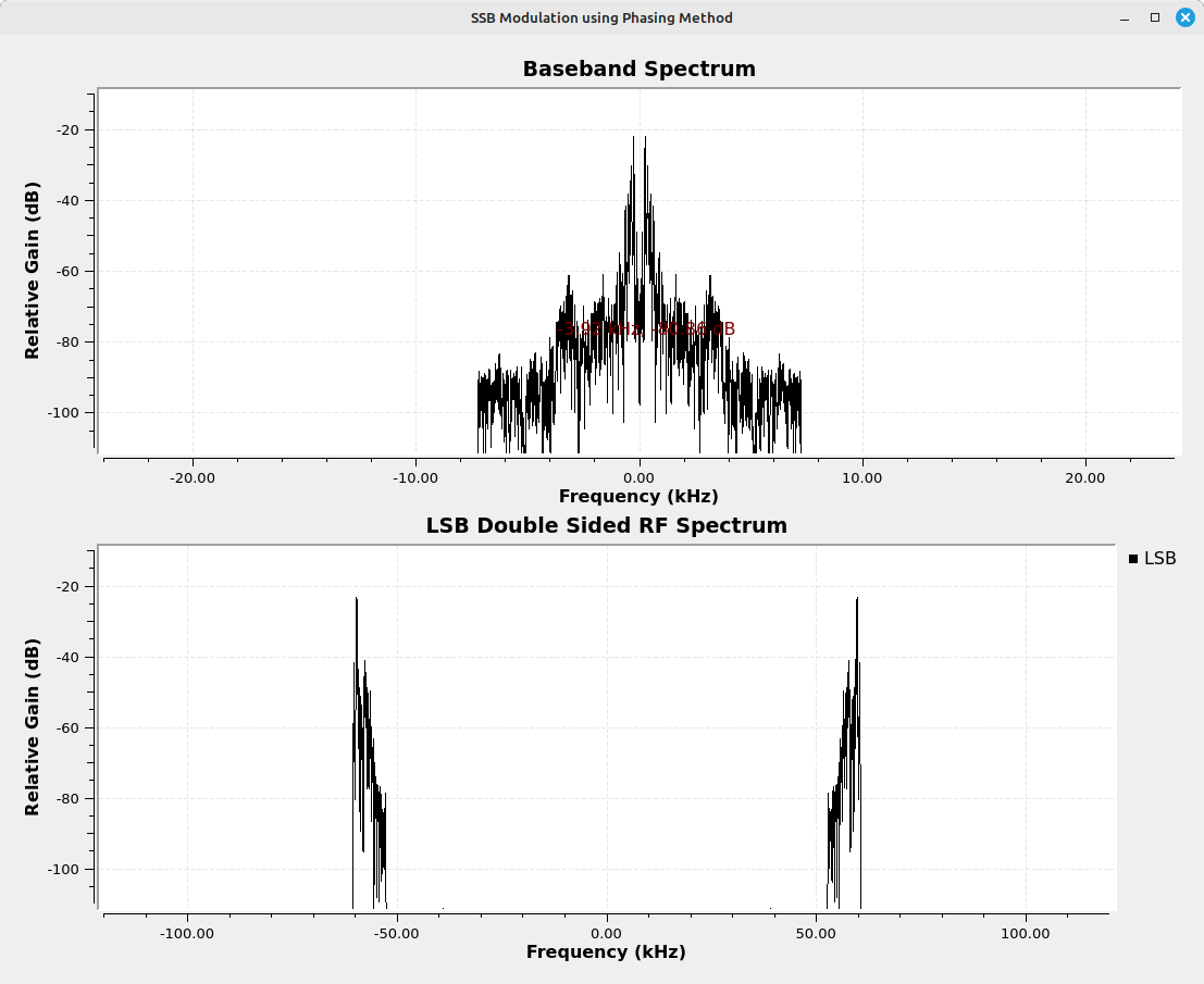
Here's a graphical way of looking at how phasing works. Near the very end, just before the add block, the phases of the two branches, I and Q, appear similar to those shown below. In the Q branch, the upper sideband is 180-degrees out of phase with the I branch upper sideband. The lower sideband is in-phase between the two. Depending on whether you add or subtract determines whether you get a LSB (add) or USB (subtract) signal.

Graphical diagram showing two double sideband signals on the left, one in the upper lefthand corner, and the other in the lower lefthand corner. The one in the lower, lefthand corner has its upper sideband flipped vertically compared to the lower sideband. Otherwise, the upper and lower signals appear the same. A plus sign is just to the right of the signals. To the right of the plus sign appears the two signals overlapped, with the words add and cancel above the overlapped signals. To the right of this is the equals sign. To the right of the equals sign is a lower sideband signal with the word LSB above it. — Diagram outlining how the phasing method works. This is how the signals would appear just before the Add block in the diagram above. Using a combination of the Hilbert transform and multiply with a complex sinusoid, the phases of the upper and lower sidebands can be either reinforced or cancelled to remove the undesired sideband. In this instance, when the two signals are added, the upper sidebands cancel between the I and Q branches, while the lower sidebands reinforce. This gives you a LSB signal.

The Hilbert Transform

You have no idea how much I wish I'd had Gnu Radio when I was an undergrad. The ability to model different things and see how they actually work is the most powerful aspect of Gnu Radio, bar none. The ability to use it to educate will be its most lasting contribution to the field of signal processing, signal analysis, and RF in general.

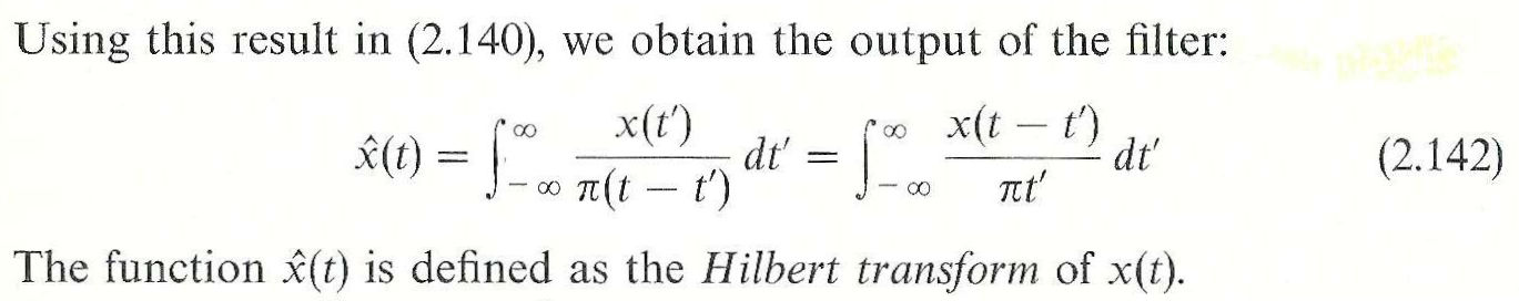
That digression is because of how I now look at the Hilbert transform. I learned about the Hilbert transform when I was an undergraduate, and the definition in the textbook was... less than helpful.

Image from an old engineering textbook that states in bold font at top 2.11 The Hilbert Transform. The next line says Definition, followed by the paragraph Consider a filter that simply phase-shifts all frequency components of its input by -pi over 2 radians; that is, its transfer function is H(f) = -j sgn f. To the right of this text it states (2.138). The bottom shows in italics 2.11 The Hilbert Transform and the page number 85. — This was how my engineering textbook began its definition of the Hilbert transform. But there are two parts here that are key for me. The first is the use of the word "filter"; the second is "phase-shifts all frequency components of its input by -pi/2 radians" (equal to -90 degrees)³.

Text from a textbook that states Using this result in (2.140), we obtain the output of the filter:. The next line is an equation that states x(t) (with a tilde over the x) equals the integral from minus infinity to plus infinity of x(t minus t prime) over the quantity x times t prime d t prime. The last line states The function x(t) (with a tilde over the x) is defined as the Hilbert transform of x(t). — Before this final equation, there is a whole derivation but this is the final definition. Again, this was... not helpful to me in understanding the Hilbert transform.

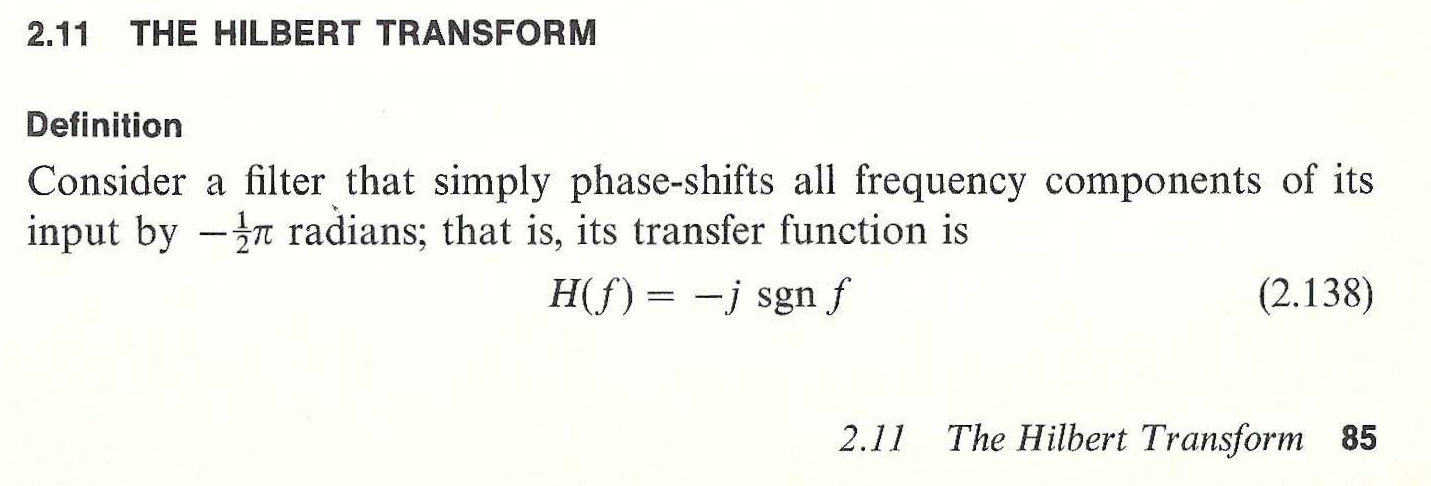
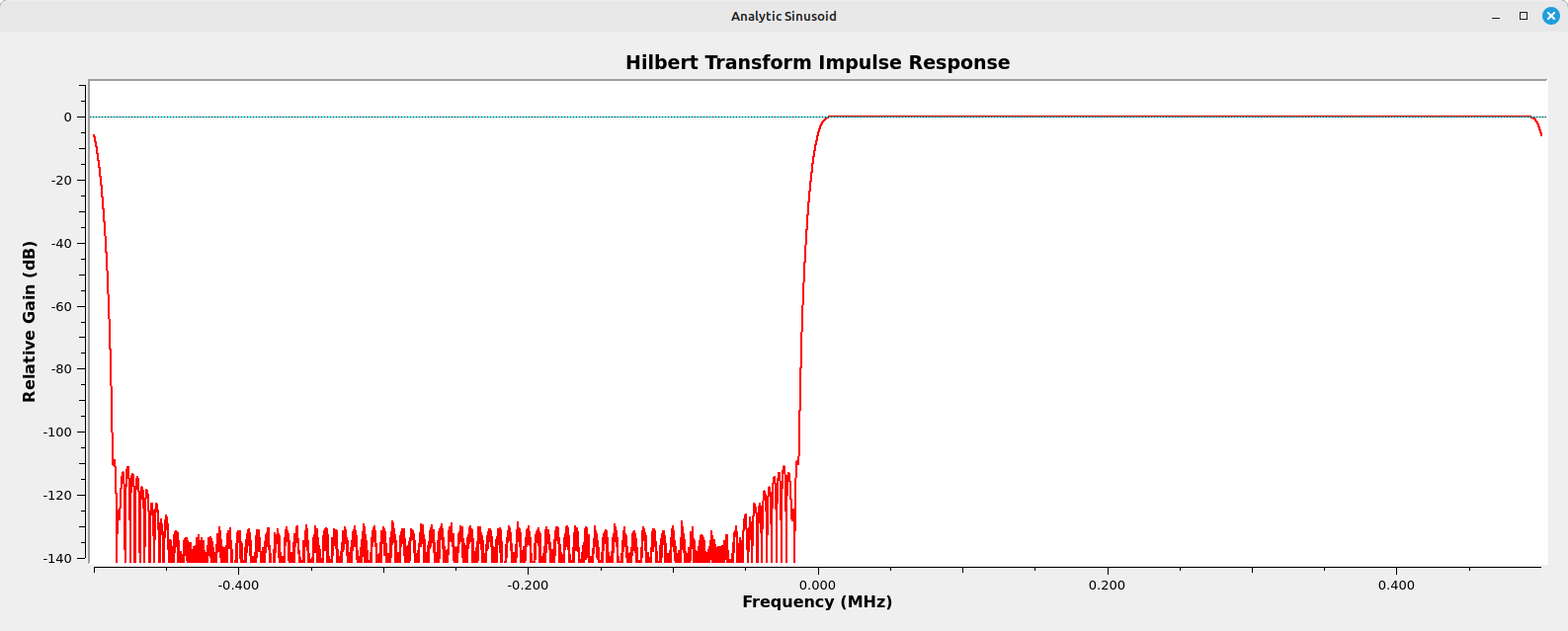
If you look at the impulse response of the Hilbert transform, specifically the spectrum of the impulse response, you see the "filter" aspect quite starkly. (NOTE: I pulled the following from my post on "soft" tuners.)

Screenshot of a block diagram for a Hilbert transform of a sinusoid. The first block creates a vector of an impulse (a bunch of zeros with one positive value) that is fed into the Hilbert transform block. The output of the transform feeds into a spectral display. — GRC flowgraph to create an impulse response for a Hilbert transform. The first block is a vector source that is a vector of 0s, but with a single, positive value in the center. That is fed into the Hilbert transform, which is really nothing more than a complex filter. This feeds into a frequency sink (spectral display) to show the spectrum of the impulse response.

Spectral display showing the impulse response of the Hilbert transform. For these particular values, the entire negative frequency portion of the spectrum has been filtered out, while the positive frequency portion is unaffected. — Spectral display of the impulse response of the Hilbert transform. Note that (almost) the entire negative frequency portion of the spectrum has been filtered out, while the positive frequency portion is unaffected. The Hilbert transform is really nothing more than a complex filter, and it is affected by the number of taps (just as with any filter) and the window type (Blackman-harris, in this case).

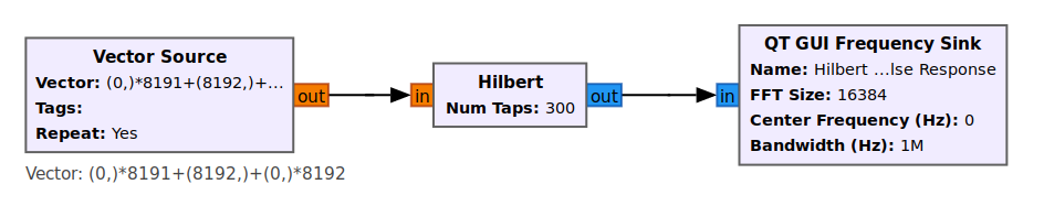
The Hilbert transform creates a complex signal. It combines the input signal, which will be the real portion, with a phase-shifted version, which is the imaginary portion. The phase shift is by -90 degrees.

One of the ways I now look at the Hilbert transform is as a bandpass filter. It removes the negative frequency components of a signal. You might disagree with that, but this works conceptually (for me, at least). But how does it do that? Well, the Hilbert transform does shift the phase of the input by -90 degrees. But that alone doesn't do anything. Let me repeat that: shifting the phase of a signal by itself doesn't do diddly-squat. If I phase shift a signal, all I've done is shift it slightly in time. Big deal. The critical part is that the phase-shifted version becomes the imaginary component, while the original signal remains as the real component. By combining the phase-shifted signal with the original, unshifted signal, we create a complex signal whose positive and negative frequencies are different. Combined, we've created an analytical signal (meaning a signal that has no negative frequency component). Therefore, any time you're using the Hilbert transform, you're also saying, "Complex signal processing to follow."

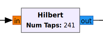
This is why when you look at the "Hilbert" block in Gnu Radio, it has a "Real" input (the orange color which GRC calls "floats"), and the output is "Complex" (the blue color). The "Hilbert" block calculates the Hilbert transform of the input and outputs it on the imaginary leg, while the original input is simply delayed equal to half of the filter taps and output on the real leg. You need both of them combined as a complex signal for the Hilbert transform to have any meaning.

Rectangular block with the words Hilbert in the center along with the words Num Taps: 241 underneath. An orange tab marked In sticks out on the left, while a blue tab marked Out sticks out on the right. — Gnu Radio Hilbert transform block. The input is real, and the output is complex.

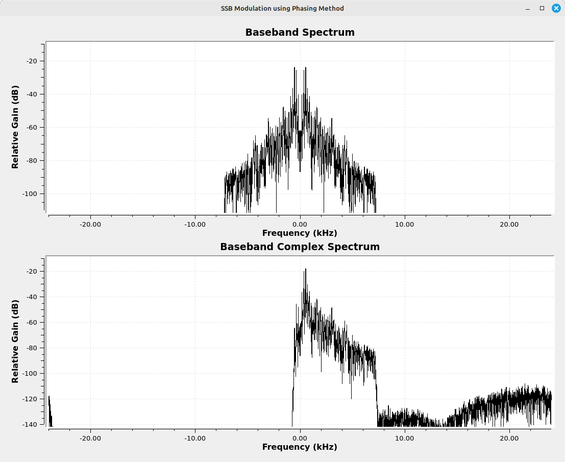
This is why there are two branches in the phasing method. It's using complex signal processing. The upper branch is the in-phase (I) branch, and the lower branch is the quadrature (Q) branch. Taken individually, each is just a real signal. Together, we can create a complex spectrum, as shown below.

A set of blocks connected from left to right. The leftmost block is an audio source feeding into a block marked Throttle, then into a block marked Hilbert. The input of the Hilbert block is orange and the output is blue. The Hilbert block feeds into a block entitled QT GUI Frequency Sink. Also connected to the output of the Throttle block is another QT GUI Frequency Sink, except it has an orange input tab, while the frequency sink block connected to the output of the Hilbert block has a blue input tab. — Gnu Radio flowgraph recreating a Hilbert transform. The output of the Hilbert transform is a complex signal, which is the only way to have unique positive and negative frequency components. Further, the only way to see these unique positive and negative frequency components is with a spectral display that uses a complex input. Hence, the QT GUI Frequency Sink is set for a complex (blue) input.

Two spectral displays, one at the top and one at the bottom. The top display shows an audio signal as double sided. The bottom display only shows the positive frequencies of the audio signal, and it now appears as a single sideband signal. — Two spectral displays of our audio signal, one before the Hilbert transform and the other after. The top display shows the double sided spectrum with both positive and negative frequencies. The signal is also still real, which is why the spectral display shows the upper and lower sidebands as symmetric (a mirror image of each other). The magnitude of the real spectrum will *always* be symmetric. The lower image is the single sided spectrum with the lower sideband effectively removed. The *only* way to see this with unique positive and negative frequencies is as a complex signal. Hence, the QT GUI Frequency Sink is using the complex (blue) input.

Finishing up the Phasing Method Modulator

We've used the Hilbert transform to give us a single sided signal. (NOTE: It's an upper sideband or USB signal right now.) Which brings us to the next issue: How does the phasing method work if it only has the one (real) output? How can we maintain this single-sided signal with only the real output? The answer is move the complex signal away from DC (0 Hz) by multiplying by a complex sinusoid. Note that this is not a complex multiply, but simply a multiply by a complex sinusoid. What's the difference? The difference is that, with a non-complex multiply by a complex sinusoid, we have to add or subtract the outputs of each branch to get the final single sideband signal. If we performed a complex multiply with our complex sinusoid, then we would only need to take the real part to get our final SSB signal.

Block diagram flowing from left to right. The first blocks are centered vertically, but after the second block, they split into two horizontal branches, one upper and one lower. The upper branch passes through three blocks, while the lower branch passes through four blocks. In the center are a set of four blocks. They combine in a final block before passing into one, last block on the far right. — Gnu Radio flowgraph demonstrating the phasing method. The audio file is split between an an upper branch (the in-phase or I branch) and a lower branch (the quadrature or Q branch). The upper branch signal is merely delayed to equal the delay of the lower branch Hilbert transform (which is nothing more than a complex filter). The lower branch Hilbert transform is converted back to real using the "Complex to Imag" (since its the imaginary component that is transformed; the real part is merely a delayed version of the input). Both sections are upsampled for the final signal. The "Signal Source" block is the local oscillator. It, too, is passed through a Hilbert transform to create the quadrature oscillator signal. Both the I and Q branches are multiplied with the I and Q phases of the local oscillator to create the upconverted (RF) signal. The "Add" block combines them to create the SSB. In this case, adding to the two together creates a LSB signal.

Two spectral displays, one over the other. The upper display shows an audio signal as a double sided spectrum, with both positive and negative frequencies present. The lower display shows the double sided spectrum of a real, lower sideband AM signal. — Spectral displays of the baseband (top) and RF (bottom) audio signal before and after SSB modulation. Both spectra are from real inputs. The reason we can now see a real spectrum of what started as a complex signal is that the signal has been moved away from DC (0 Hz).

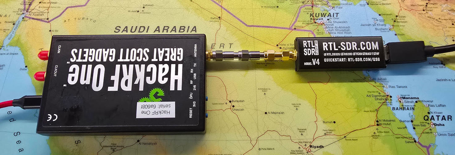
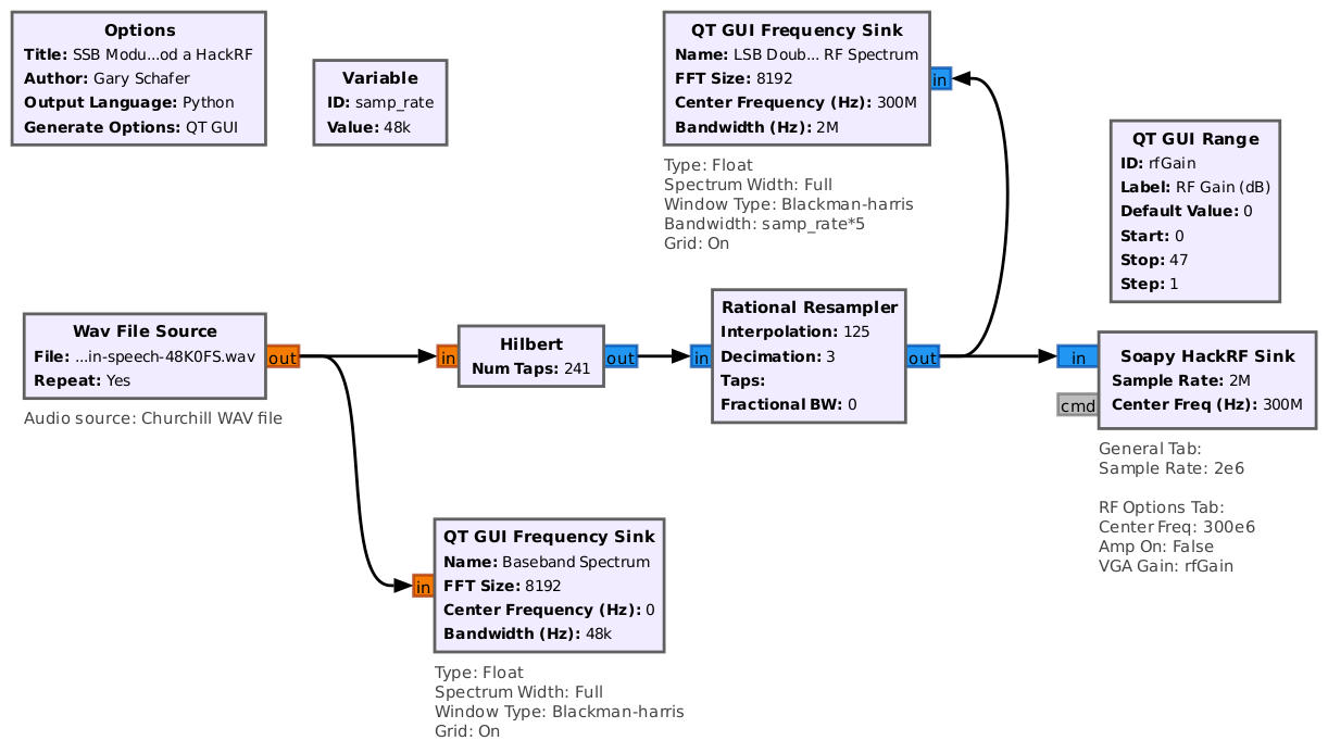
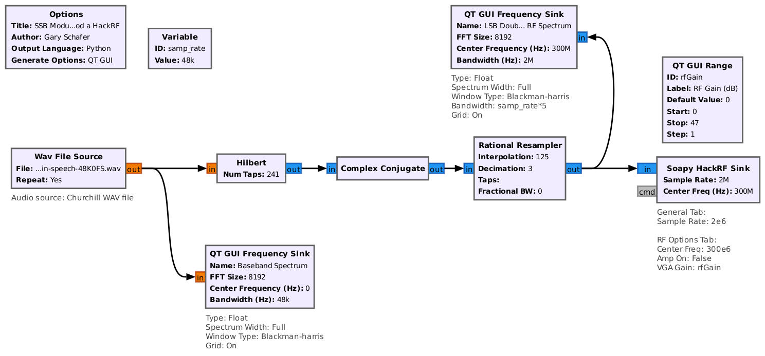
How would this work with a SDR? I setup a HackRF connected directly to a RTL-SDR, then I adjusted the Gnu Radio flowgraph to account for this. Gnu Radio input the audio signal and passed it through the Hilbert transform. The output goes directly to the HackRF through the "Soapy HackRF Sink". To keep me in the good graces of the FCC, I connected the HackRF directly to a RTL-SDR through a series of SMA attenuators.

Overhead view of a HackRF on the left connected to a RTL-SDR on the right. The connection in between is a series of SMA attenuators and an adapter. USB cables connect the HackRF from the left and the RTL-SDR from the right. — The HackRF is the transmitter and is connected directly to a RTL-SDR through a series of SMA attenuators and a SMA male-to-male adapter.

Block diagram with dashed lines forming two areas, one on the left and one on the right. The left box is entitled Gnu Radio. The right box is entitled HackRF. The whole image is entitled Phasing Method Transmitter with HackRF. — Block diagram of the phasing method transmitter broken down into two sections. The first section is the part Gnu Radio processes. The other section is the portion that the HackRF processes.

Block diagram showing a signal flow from left to right. An audio signal is input on the left, passes through a Hilbert transform, is upsampled, then passes into a HackRF. Two frequency displays show the signal at various points in the flow. — Gnu Radio flowgraph showing how the phasing method works with an actual SDR. Gnu Radio inputs the audio and performs the Hilbert transform. The signal is passed as a complex signal to the HackRF. The internal workings of the HackRF provide the multiplication by the complex sinusoid.

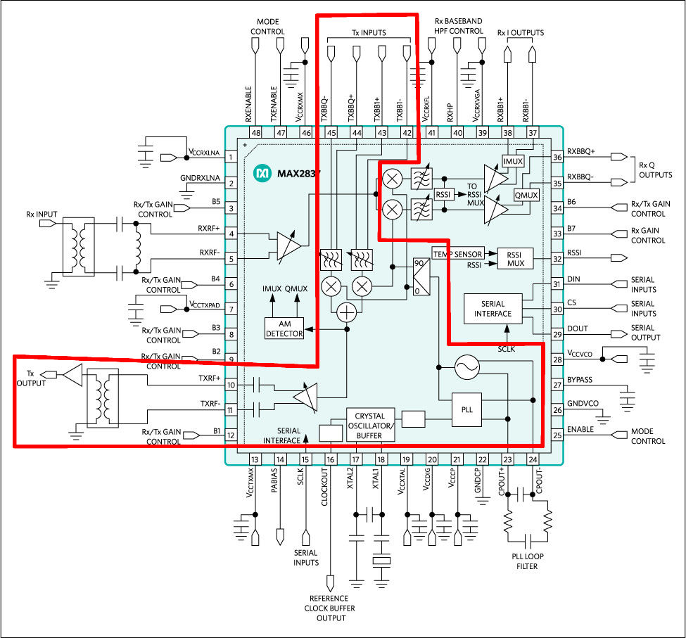
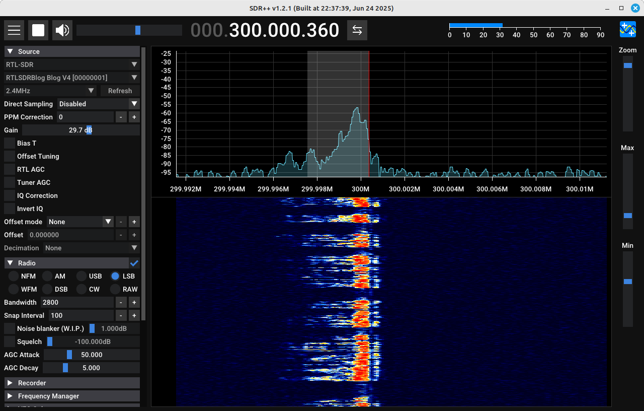
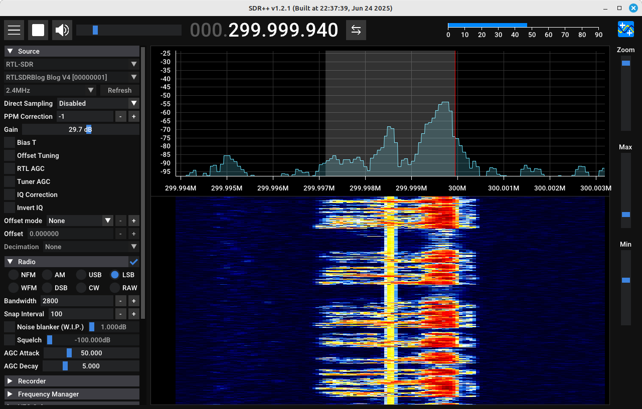
Looking at the chip that the HackRF uses for quadrature modulation (from complex to real), the Maxim Integrated MAX2837 chip, the block diagram seems to show the exact, same setup as with the Gnu Radio flowgraph of multiplication by the complex sinusoid. To confirm the output, I used SDR++.

Complicated block diagram with connections on all four sides. Each side has 12 connections, with various schematics surrounding it. The interior is a block diagram showing the signal processing between connections. A red line surrounds a portion of the diagram. — Block diagram of the Maxim Integrated Products MAX2837 chip. This chip creates the complex sinusoid and multiplies each branch (I and Q) with each portion of the complex sinusoid. In this diagram, the I portion is offset from the Q portion by +90 degrees. This is equivalent to setting the Q portion to -90 degrees with respect to the I portion. The output of the two mixers are added together. This means that this particular circuit is equal to summing (adding) the two branches together. (Block diagram image credit: Maxim Integrated Products, Inc.)

Screenshot of a software defined radio showing a spectral trace on top and a spectrogram on the bottom. The trace and spectrogram show an upper sideband amplitude modulated signal. Along the left is a column showing various parameters of the SDR, including the gain, the demodulator, and a section for recording the signal. — SDR++ screenshot showing the single sideband signal. Note that the signal is upper sideband, even though the phasing method demonstration with Gnu Radio said that summing the two branches (I and Q) should create a lower sideband. This would indicate that, somewhere in the signal path of the HackRF, the Q branch is inverted.

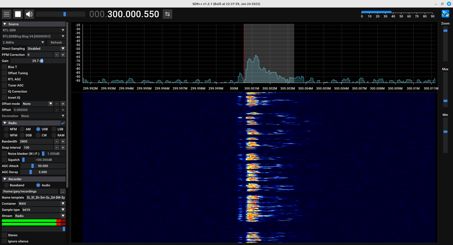
You may have noticed that the HackRF doesn't flip the spectrum as did the Gnu Radio demonstration of the phasing method. That's because of how most SDRs work. They take a complex input and essentially frequency shift it to the desired frequency. When someone sets up the input, they can see what goes into the SDR. It doesn't make sense to have the RF signal coming out of the SDR be a spectrally-flipped version of what went in. This will confuse the users. It's best to ensure that how the signal went in is the same as how it comes out.

Since the HackRF is not flipping the spectrum as does the original Gnu Radio flowgraph, in order to create a LSB signal, we need to flip the sign of the imaginary component. This is a complex conjugate. Adding one of those into the flowgraph, and we get a lower sideband (LSB) signal.

Block diagram showing a signal flow from left to right. An audio signal is input on the left, passes through a Hilbert transform, followed by a complex conjugate, is upsampled, then passes into a HackRF. Two frequency displays show the signal at various points in the flow. — Gnu Radio flowgraph for creating a lower sideband (LSB) signal with the HackRF. The audio signal passes through the Hilbert transform followed by a complex conjugate. By the magic of math, flipping the sign of the imaginary component (which is what the complex conjugate does) creates a mirror image of the spectrum. Hence, a USB signal becomes a LSB signal, and vice-versa. Since the Hilbert transform creates a USB signal, the output of the complex conjugate will be a LSB signal.

Screenshot of a software defined radio showing a spectral trace on top and a spectrogram on the bottom. The trace and spectrogram show a lower sideband amplitude modulated signal. Along the left is a column showing various parameters of the SDR, including the gain, the demodulator, and a section for recording the signal. — SDR++ showing the spectral trace (top) and spectrogram (bottom) of the lower sideband signal created in Gnu Radio.

Weaver Method Modulator

In 1956, an engineer, DK Weaver, created yet another method, which he called the "third method", for generating SSB signals. In my opinion, his method was a combination of the first two, using aspects of both the filtering and the phasing methods. It uses two multiplications of complex sinusoids, with a filtering in the middle.

Block diagram showing an input on the left and output on the right. The input splits into two branches, one along the top and one along the bottom. On the left is a vertical column representing a multiplication by a complex sinusoid, along with a similar column on the right. In the center is a vertical column representing lowpass filters for each branch. — Block diagram showing SSB modulation using the Weaver method. The input on the left is split into two branches, an I and Q. This is similar to the phasing method. The difference is that, rather than starting with a Hilbert transform on the imaginary branch, the signal is multiplied by a complex sinusoid. Because the original signal is real, the multiplication with the complex sinusoid is equivalent to a complex multiply. This means the spectrum will be shifted (to the right for a positive frequency shift; to the left for a negative frequency shift). The first multiplication with the complex sinusoid is by *half of the signal bandwidth* (typically 1200 - 1500 Hz). It's also a positive frequency shift.

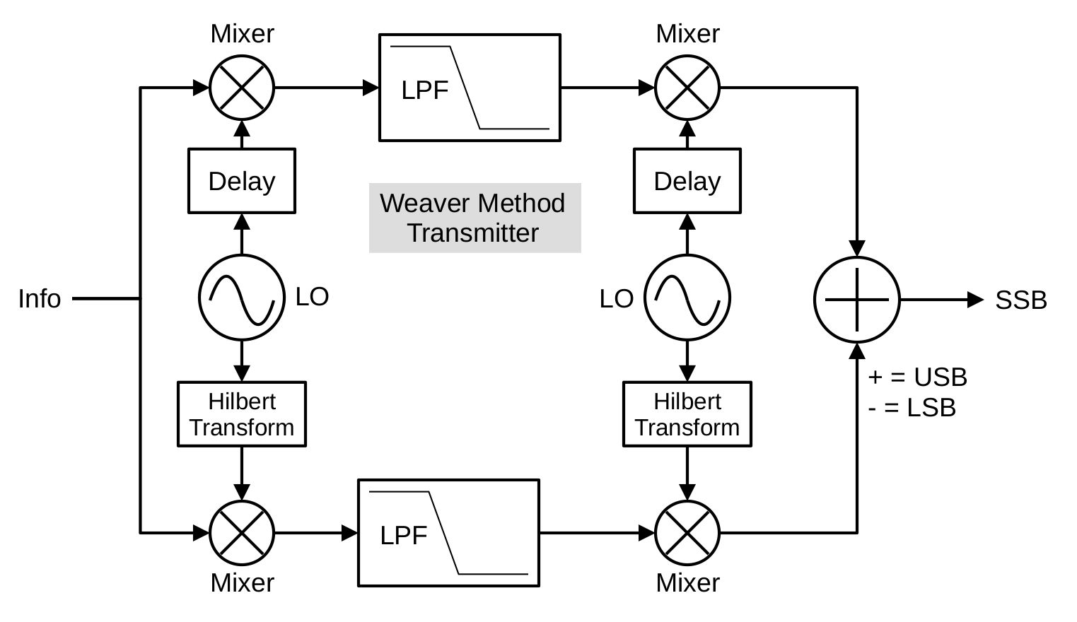
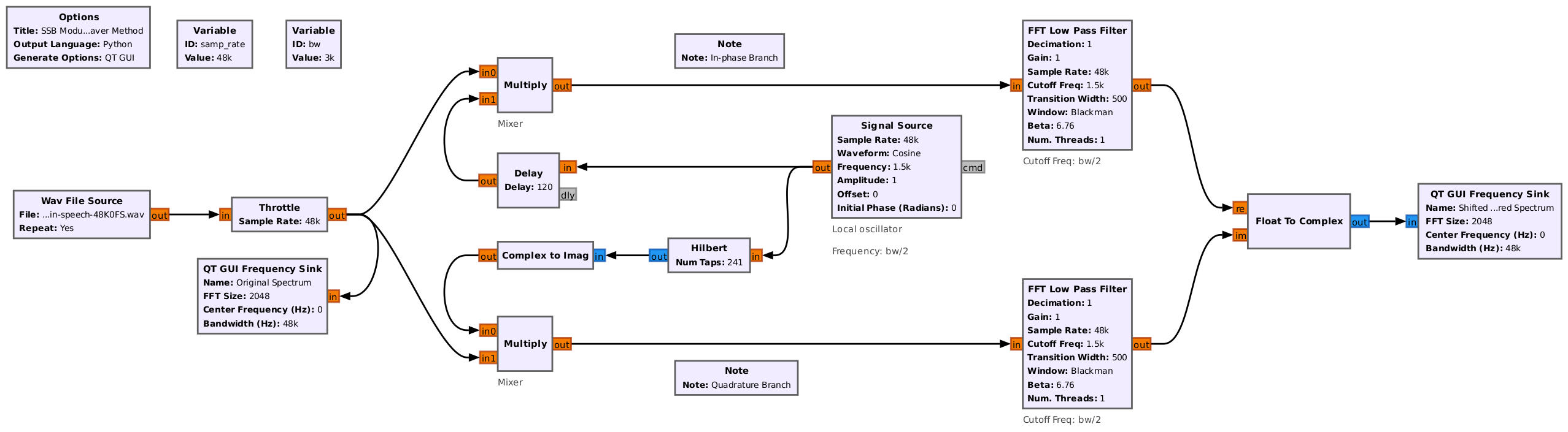
Let's look at this one section at a time. As stated, the first set of mixers multiply the incoming audio signal with a complex sinusoid. This is a complex multiply with a complex sinusoid because the input signal is real-only.

Block diagram showing a signal flow. The signal enters on the left then splits into two, horizontal branches, one along the top and the other along the bottom. Each branch passes through a multiplication block. Each multiplication block is fed be the input signal at one input, and by either a cosine or a sine wave at the other input. The output passes into a spectral display. There's also another spectral display to show the signal when it first enters the flow. — Gnu Radio flowgraph showing the input signal after it has passed through the first multiply by the complex sinusoid.

Two spectral displays, one over the other. The top display shows the double sided spectrum of an audio signal. The bottom display shows the same spectrum, only shifted slightly higher in frequency. — Spectral displays showing the double sided spectrum of the audio signal (top), and after it has been multiplied by the complex sinusoid (bottom). Note that the lower sideband is now centered at 0 Hz (DC).

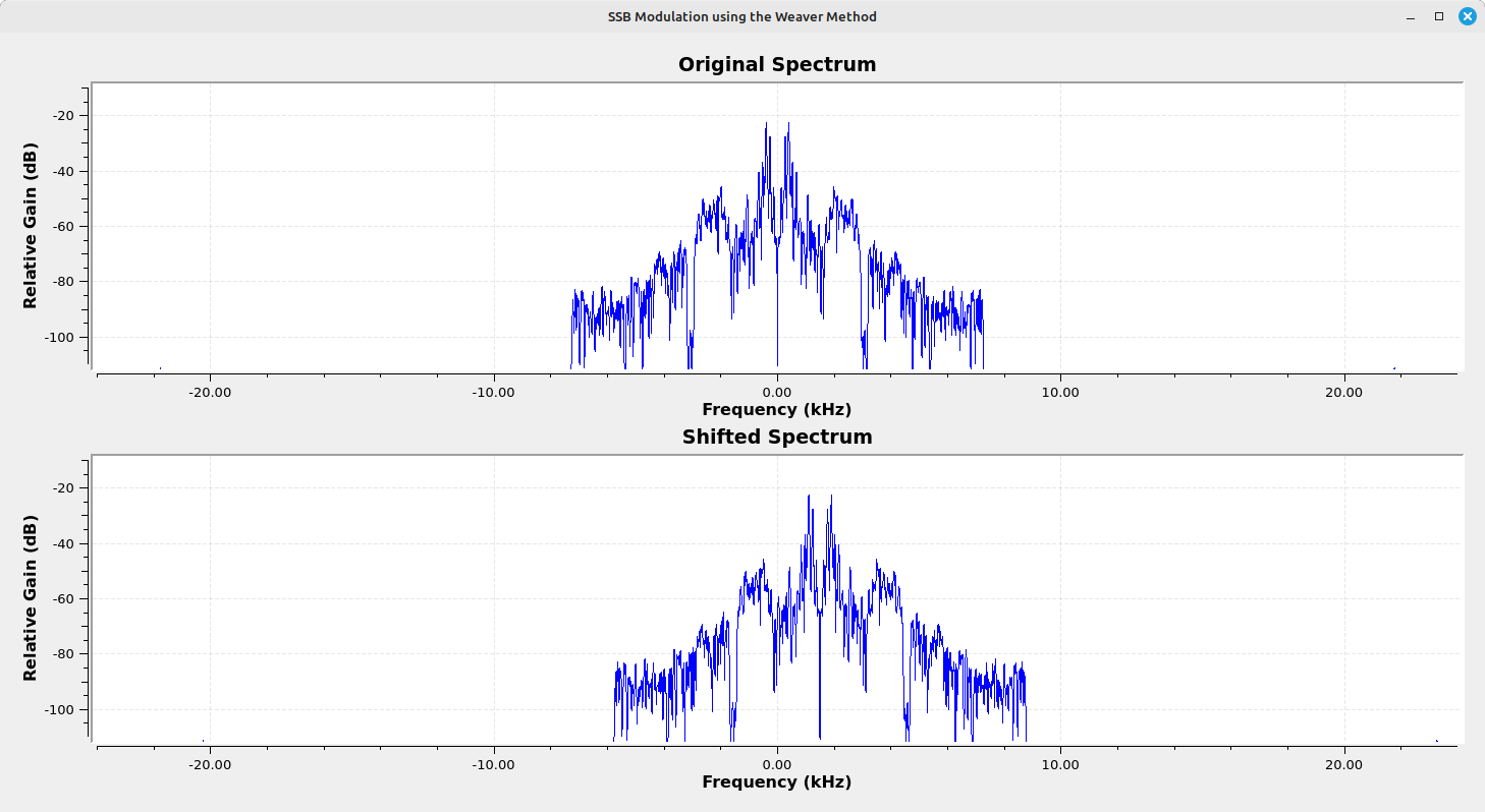
With the lower sideband now centered at 0 Hz, we'll add the lowpass filters. With the sideband centered, the lowpass filter will only pass that sideband and remove the other. Note that the addition of the lowpass filters along with the multiplication by the complex sinusoid creates a quadrature demodulator, a standard circuit for creating a complex signal from a real one.

Block diagram showing an input audio signal on the left, then splitting into two, horizontal branches along the top and bottom. Each branch passes through a multiplier followed by a lowpass filter. The multipliers are also tied to either a cosine wave on the top branch, or a sine wave on the bottom branch. The outputs are passed into a frequency display as a single, complex signal. — Gnu Radio flowgraph that both multiplies the input signal with a complex sinusoid, then filters each branch (I and Q). This is a quadrature demodulator, a standard circuit for converting a real signal into a complex one.

Two spectral displays, one over the other. The top display shows the double sided spectrum of the original audio signal. The bottom display shows the signal after it has been filtered, which is a lower sideband signal centered at 0 Hz. — Spectral displays showing the original audio signal (top) and the now-filtered lower sideband signal centered at 0 Hz (bottom).

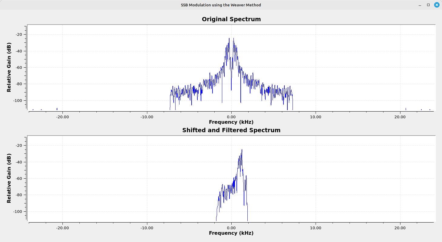
The last part is to once-again multiply this complex signal with a complex sinusoid. Now, since this is not a complex multiply with the complex sinusoid, either of the signals separately will be worthless. The signals have to be combined. Specifically, they have to be added to create the final RF signal.

Block diagram showing an input signal on the left. The input splits between two, horizontal branches. One branch runs along the top, and the other branch runs along the bottom. Each branch passes through a multiplier, a lowpass filter, then another multiplier. The first multiplier shifts the signal by half of the bandwidth. The lowpass filter passes only one sideband. The second multiplier shifts to the RF center frequency. — Gnu Radio flowgraph demonstrating the full Weaver method. The audio signal is split between an upper branch (I) and a lower branch (Q). The first set of Multiply blocks shifts the signal higher by half of the output bandwidth. The bandwidth, in this example, is set to 3 kHz. The shift is therefore 1500 Hz. The output of the shifted spectrum passes through lowpass filters. These only pass the lower sideband, removing the upper sideband. The next set of Multiply blocks shift the complex signal to the final, RF center frequency. Because this is *not* a complex multiply, the signals have to be combined to create the final signal. That's the purpose of the final Add block.

Two spectral displays, one over the other. A set of two buttons are arrayed along the top, horizontally. The top display shows the double sided spectrum of the original audio signal. The bottom display shows the single sideband RF spectrum. — Spectral displays of the original audio signal (top) and the SSB signal in the RF spectrum (bottom).

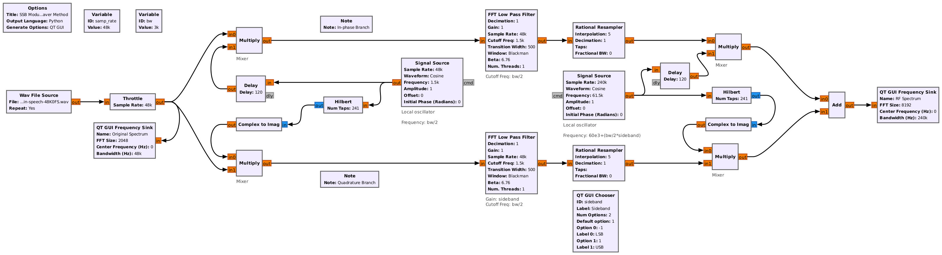
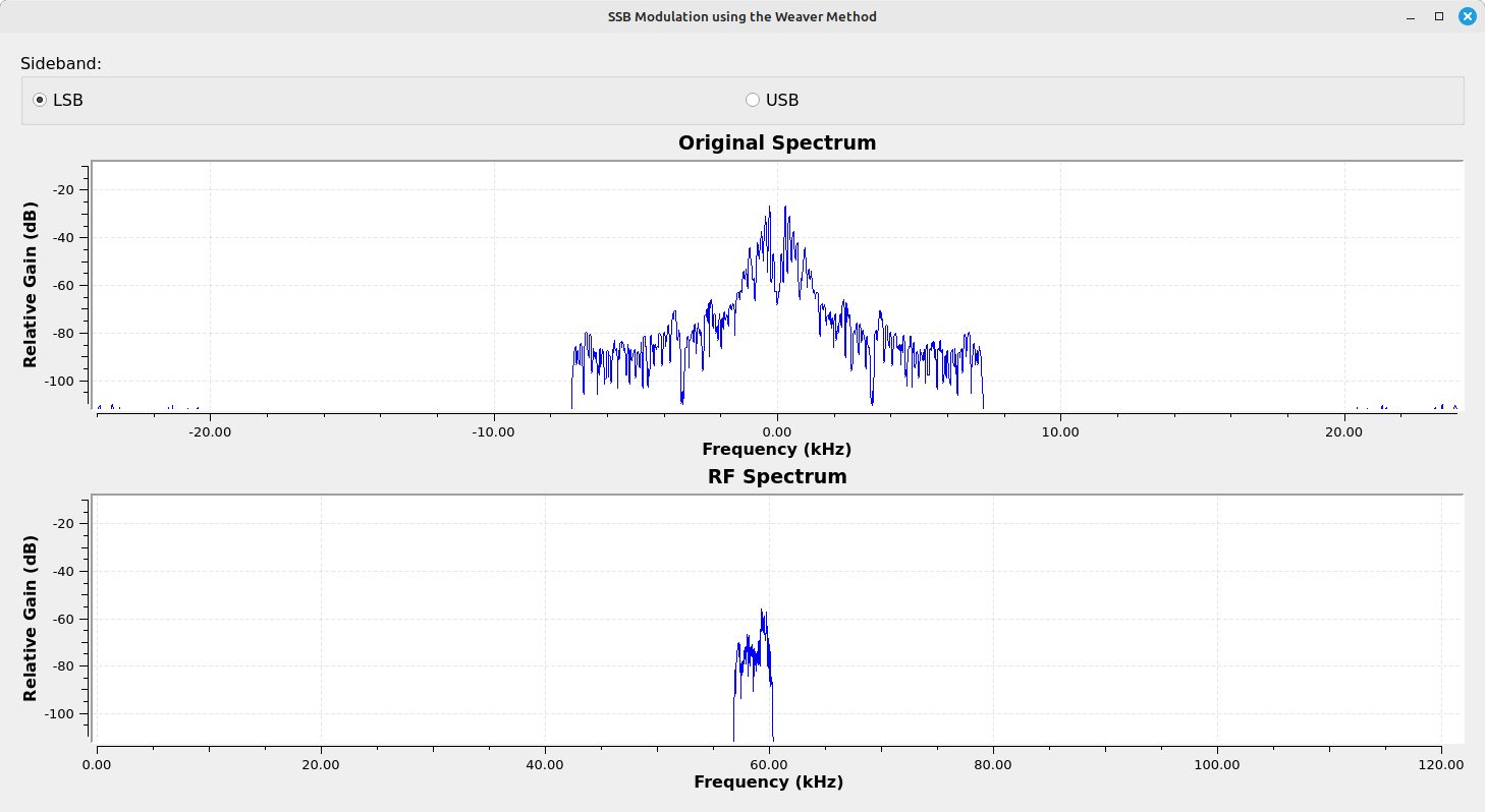
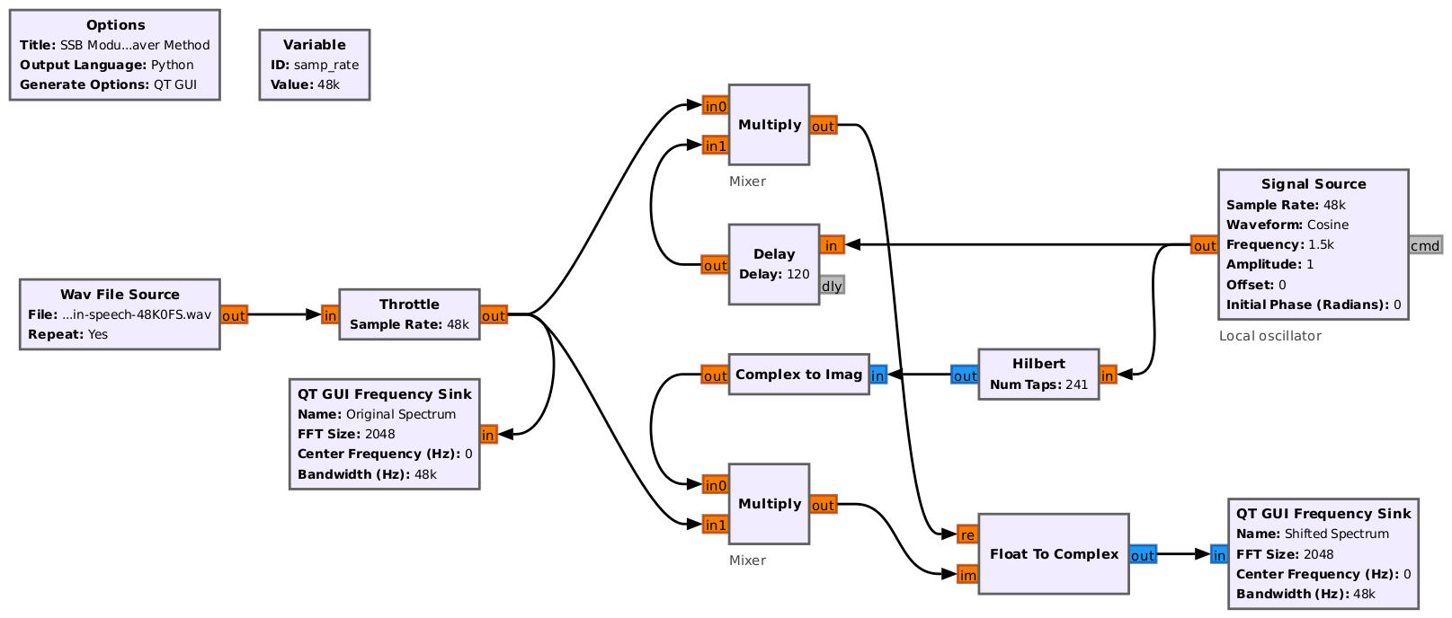
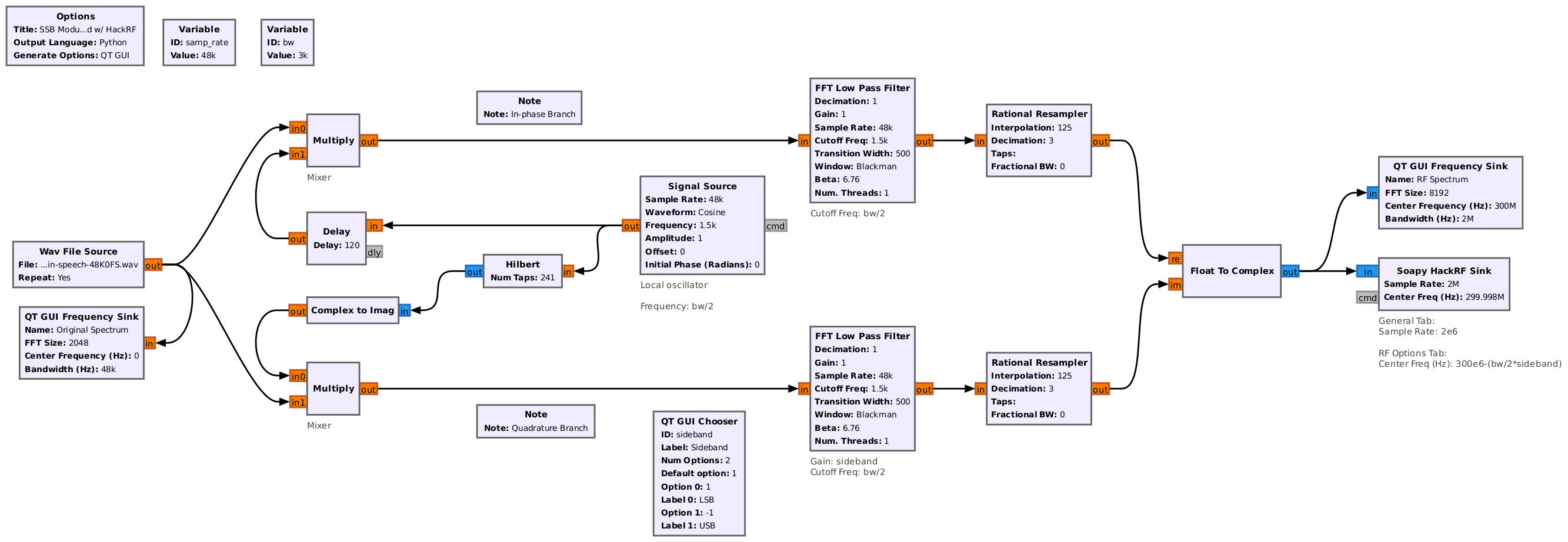
Let's break up the original block diagram to define what Gnu Radio will do, processing-wise, and what the transmitter (the HackRF) will do.

Block diagram with a signal flow going from left to right. The audio input starts on the left, then splits into two, horizontal branches, an upper one and a lower one. The signal passes through a multiplier and lowpass filter in each branch. The output of each branch is combined as a single complex signal, then is passed into a block marked HackRF. Parallel with the HackRF block is a block for displaying the spectrum. — Block diagram using the Weaver method and going into a HackRF. The signal is split, multiplied by a complex sinusoid, and filtered. Effectively, this is passing the signal through a quadrature demodulator. The complex output is sent into the input of a HackRF for transmission.

Block diagram similar to the previous one, with the final output connected to a HackRF sink block. — Gnu Radio flowgraph using the Weaver method for the first, two sections (multiply by complex sinusoid and filter), which is then input into a HackRF.

Screenshot of the SDR control program SDR++. Along the left is a column of various controls. Along the top is a start button and a set of numbers to set the center frequency. The majority of the screen is covered with a spectral trace along the top, and a spectrogram along the lower half. A lower sideband signal is displayed in both the spectral trace and the spectrogram. — SDR++ display of a lower sideband transmission using the Weaver method into a HackRF. Note that the center of the sideband has the LO feedthrough signal. This is an issue of the Weaver method, unless a complex frequency shift is applied before going into the SDR. This would only add to the complexity of the transmitter.

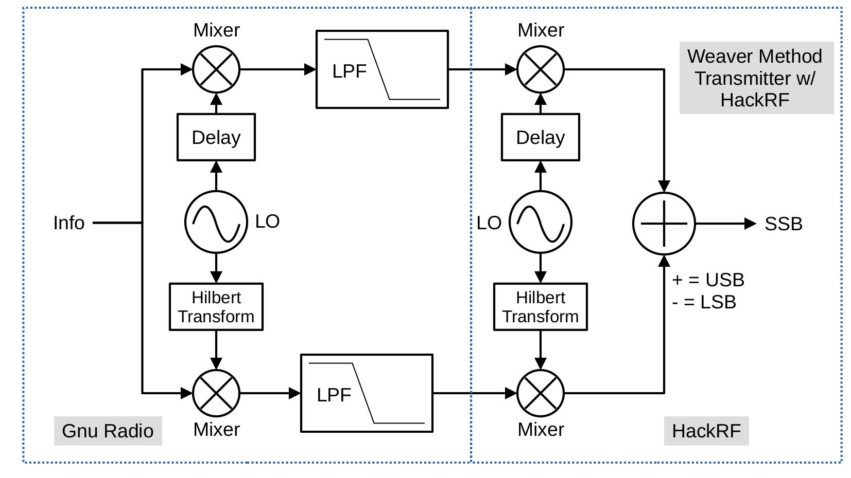
The Weaver method means that, unless you add yet another frequency shift (and a complex one, at that, which is much more complicated for real-only signals), we wind up with a signal that is directly at the center frequency of the transmitting SDR. Which is where most SDRs have a spike from the LO feedthrough. Not a great look.

SSB Demodulation

Now that we know how to modulate SSB signals with various analog techniques, let's look at some analog techniques for demodulation. We'll cover the same three we used for modulation, specifically filtering, phasing and Weaver.

Filtering Method Demodulator

This is straightforward. Use a narrowband filter to only pass the desired sideband, apply a coherent recovery circuit (namely, a beat frequency oscillator or BFO), and you have the original signal back.

Block diagram showing a signal flowing from left to right. The left-most, input block is a file, which passes through a Throttle block, then is split between two bandpass filters. The upper bandpass filter is marked for the lower sideband, while the lower block is marked for the upper sideband. The outputs of the filters connect into a block used to select the desired sideband. The selector output connects to a multiplier and signal source, and is marked beat frequency oscillator. The output of the multiplier connects to a lowpass filter, followed by an audio output. — Gnu Radio flowgraph demonstrating a filter-based SSB receiver. The flowgraph has separate bandpass filters for the upper and lower sidebands, with a selector block used to select the appropriate one. The Signal Source block along with the Multiply block acts as a real signal mixer. Since it's a real (as opposed to complex), it has to be followed by a lowpass filter to select the difference frequency. The output of the filter is the demodulated signal and can be input to the Audio Sink block.

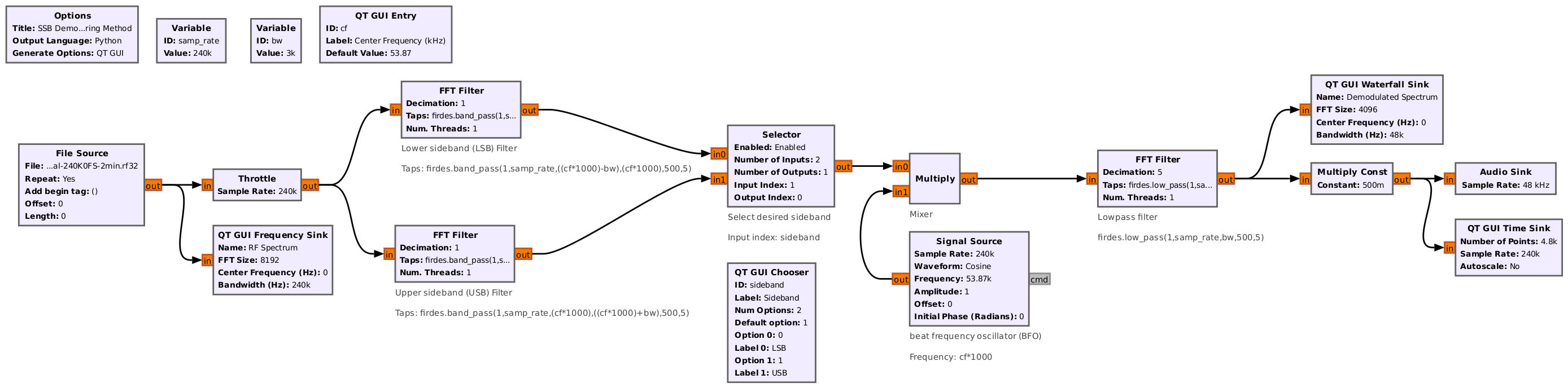
This basic demodulator can also handle either SSB or ISB. It has the advantage of simplicity (no balanced mixers required, no need for Hilbert transforms), but the downside (from an analog sense) would be the requirement for a relatively high-Q filter (that's "Q" as in "quality factor" for analog filters, not "Q" as in "quadrature").

I didn't modify this to work with an actual SDR. Instead, I'm going to demonstrate a filtering-method demodulator using complex signal processing at the end of this post.

Phasing Method Demodulator

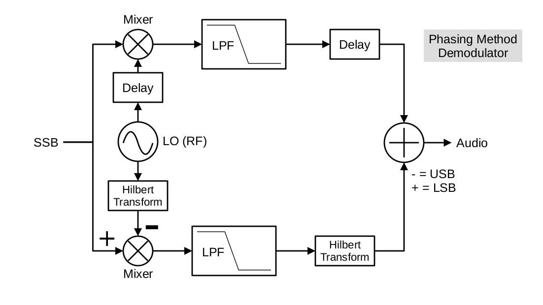
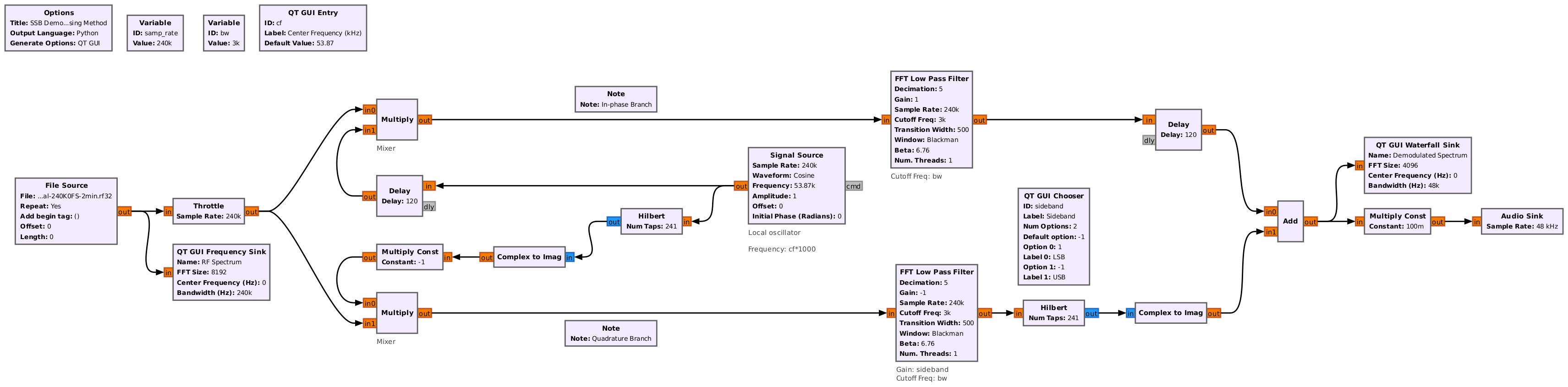
The phasing method demodulator is effectively the phasing method modulator in reverse. The diagram below is based on Rick Lyon's paper on the phasing method⁴.

Block diagram showing a SSB signal input on the left, then being split between two, horizontal branches, one along the top and the other along the bottom. Each branch is multiplied with a sinusoid (forming a complex sinusoid), followed by a lowpass filter. The lower branch, marked as the quadrature branch, passes through a Hilbert transform. The top branch passes through a delay that aligns with the transform. Both branches are put into an add block before passing into a spectral display and audio output. — Block diagram of a phasing method demodulator. The input signal, which is real, is downshifted using a complex multiply with a complex sinusoid. This will both convert the input signal into complex, and also center it at DC (0 Hz). Each branch, I and Q, passes through a lowpass filter. This creates a filtered, complex signal with either the USB, LSB or ISB signal. The complex signal goes through a Hilbert transform. Each branch of the complex signal is summed to create the final audio signal. A Multiply Const block on the quadrature branch inverts the Q branch for USB; otherwise, the sum will create a LSB signal. Note that this will also work on an ISB signals.

Gnu Radio flowgraph consisting of blocks flowing from left to right. The left most block is a file source reading in the signal. It passes through a throttle block, then splits into two, horizontal branches. One branch runs along the top, while the other runs along the bottom. Each branch multiplies the signal with a complex sinusoid, then is filtered, and the resulting complex signal passes through a Hilbert transform. The final block sums the top and bottom branches to demodulate a LSB signal, while subtracting them creates a USB signal. The output on the right is sent to a spectral display and audio output. — Gnu Radio flowgraph showing a demonstration for a SSB demodulator using the phasing method. The input signal (a file containing samples of a SSB signal stored as real samples) is split and multiplied with a complex sinusoid. This effectively downshifts the signal to DC (0 Hz). The output is filtered, and the quadrature branch passes through a Hilbert transform. The two branches are summed to fully demodulate the signal. If the sum is positive, the demodulated portion will be the LSB; if the sum is negative (subtraction), the demodulated portioned will be the USB.

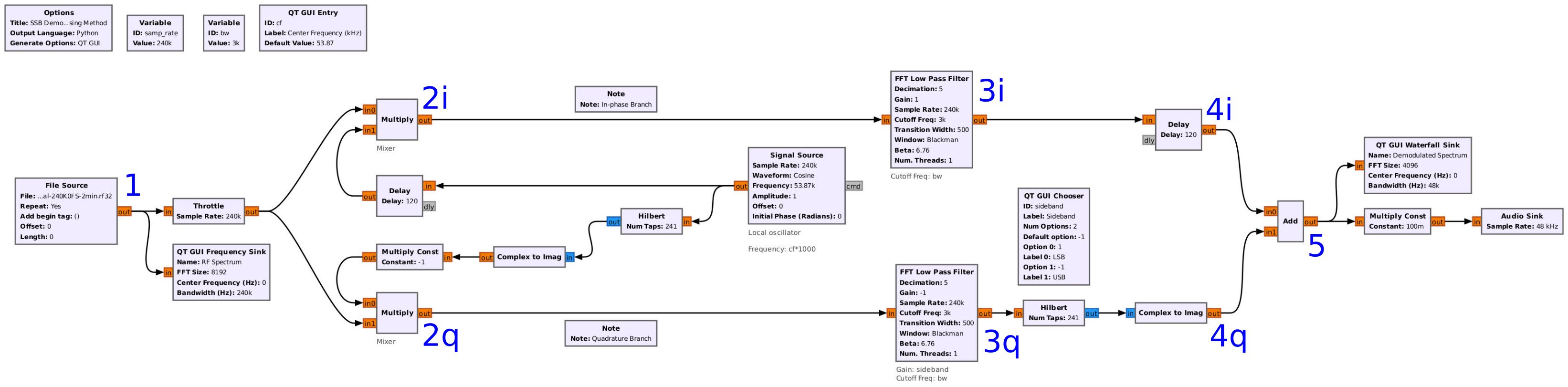
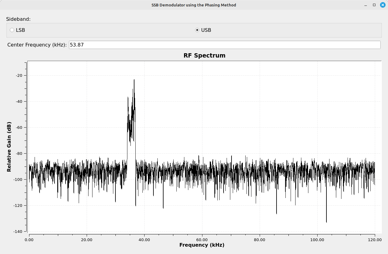
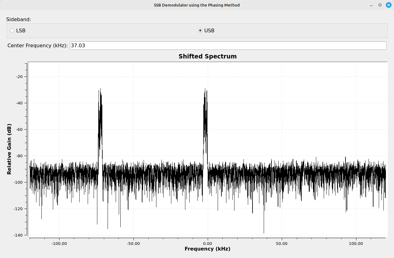
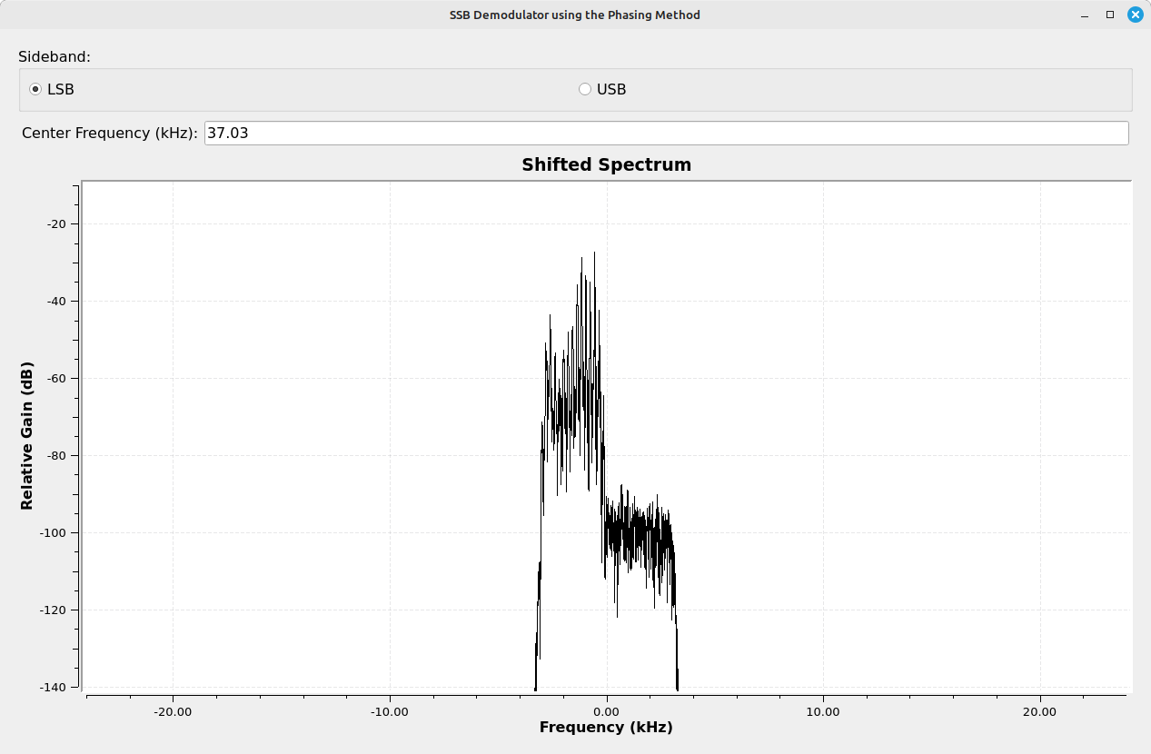
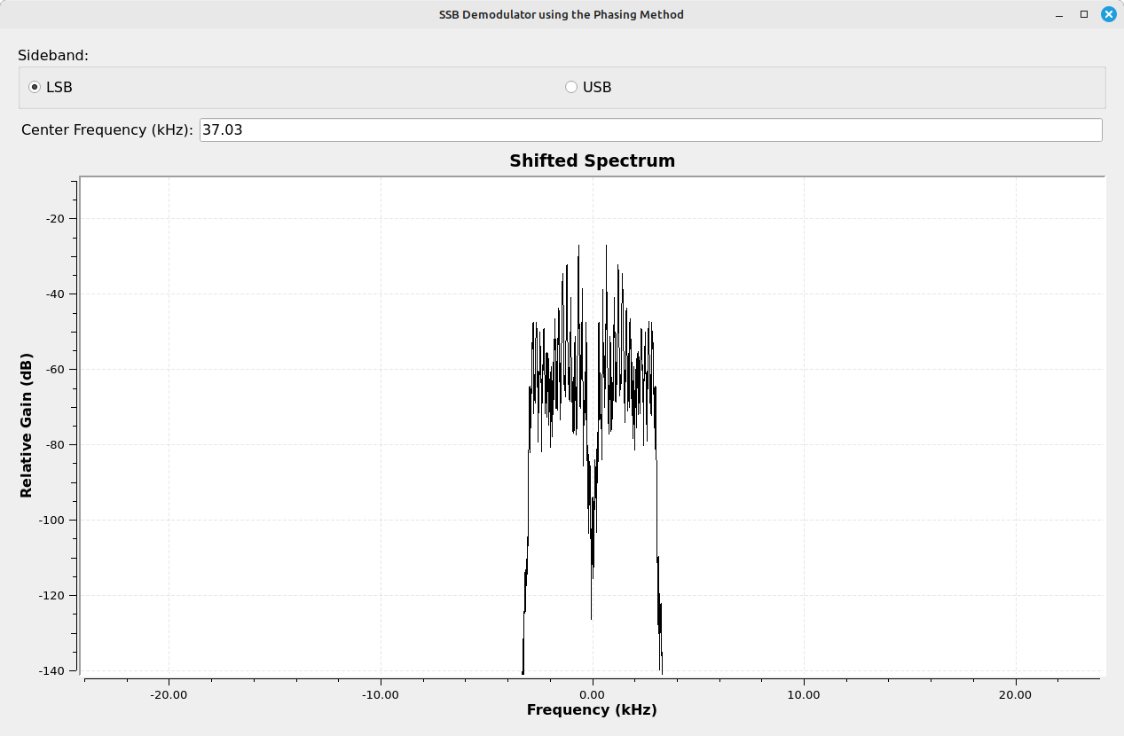
Let's take a look at the signal at different points in the Gnu Radio flowgraph to see how it changes at each stage. For this, we'll use the following points (numbered 1 - 5), with the corresponding spectral display at each point.

Block diagram flowing from left to right. The input is a file on the left. After passing through a block marked Throttle towards the right, it splits into two, horizontal branches. One branch runs along the top and the other along the bottom. Each branch passes through a multiplier (with the outputs marked 1i and 1q, respectively, between top and bottom), and then a lowpass filter block (with outputs marked 2i and 2q between top and bottom, respectively). Along the top branch, the output of the lowpass filter connects to a block marked Delay, and with the value 3i on its output. The lower branch output of the lowpass filter connects to a block marked Hilbert transform followed by a block marked Complex to Imaginary and whose output is marked 3q. The outputs marked 3i and 3q both connect to a block marked Add, whose output is marked 4. That output connects to a spectral display and audio output. Back near the left side, a block marked signal source connects to each of the multiplier blocks after passing through a Delay block (upper branch) and Hilbert transform and Complex to Imag block (lower branch). — Annotated block diagram showing the points where we can look at the spectrum of the signal as it flows through different stages of the phasing demodulator.

Spectral display showing a LSB signal. — Point #1) Spectral display showing the original, RF signal. This is a LSB signal.

Spectral display showing the RF spectrum after the signal has been shifted by the complex sinusoid. — Point #2) This is the complex spectrum of the signal after it has been shifted. The positive frequency signal has been shifted to 0 Hz.

Spectral display showing a lower sideband, single sideband signal centered at 0 Hz. — Point #3) This is the complex spectrum after passing through the lowpass filters. The single sideband signal (whether USB or LSB) is now centered at 0 Hz. This is the spectrum of a LSB signal.

Spectral display showing a double-sided spectrum of a signal. — Point #4) This is the complex spectrum of the signal after it has passed through the Hilbert transform. Note that it appears to be just a basic, double-sided AM signal. It's not. The spectral display shows the *magnitude* of the signal, but not how its phase differs between the positive and negative frequencies. Regardless of whether the user selects USB or LSB (which does change how the signal is processed), this spectrum would appear the same.

Spectrogram (spectral waterfall) display showing a strong signal along the left edge at the top half of the screen, then no signal along the bottom half. — Point 5) A spectrogram (aka "waterfall" or "rising raster") showing the final, demodulated output after adding the I and Q branches together. The original signal was LSB (lower sideband), and selecting that option means that the two branches are added together. When selecting USB (upper sideband), the Q branch is subtracted from the I branch. Because of the various phases of the positive and negative frequencies, selecting USB when the signal is LSB means that you get... nothing.

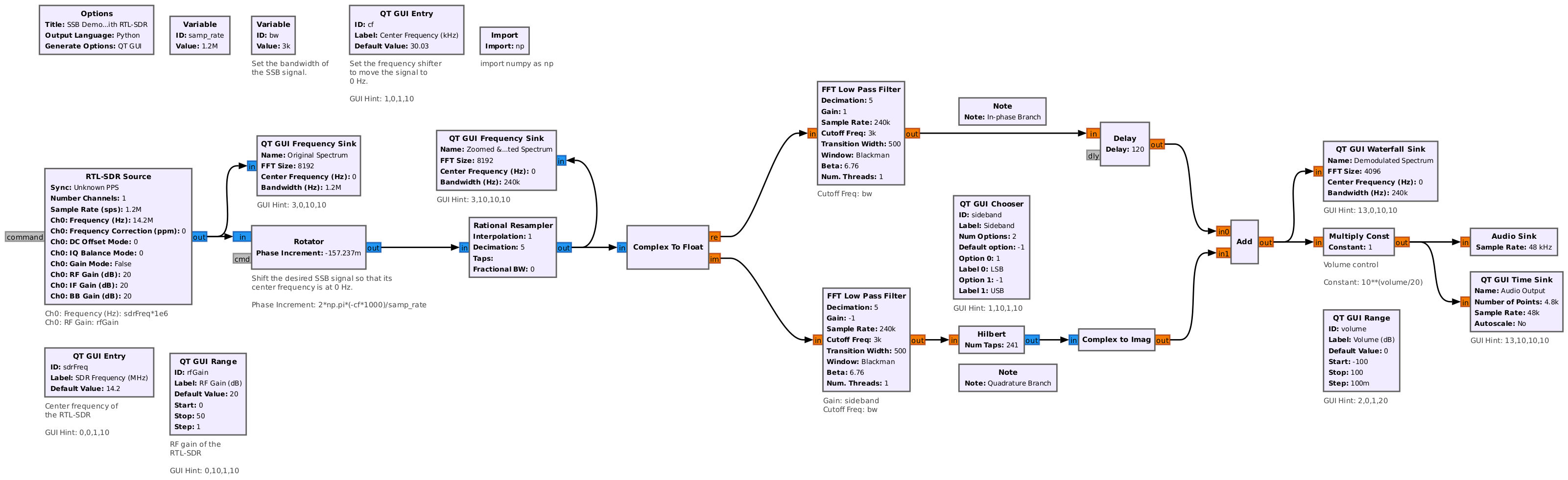
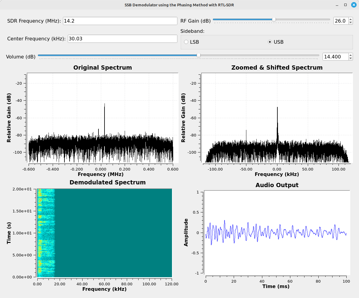
Here's how it looked when I modified the flowgraph to work with a RTL-SDR. Once again, I used the HackRF One to generate the SSB signal while using the RTL-SDR to receive it.

Block diagram for signal processing flowing from left to right. The first block on the left is marked RTL-SDR source. It connects to a block marked Rotator, which itself connects to a block marked Rational Resampler. The output of the resampler connects to a block marked Complex to Float. The output of this block splits between two, horizontal branches, one upper and one lower. Both branches pass through a filter, while the upper then passes through a delay and the lower passes through a Hilbert transform and complex to imaginary. The two branches are summed (connect to an Add block), then pass into a time sink, spectral display and audio output. — Gnu Radio flowgraph implementing the phasing method demodulator using a RTL-SDR. Note that the RTL-SDR is providing the initial mixing with a complex sinusoid. The Gnu Radio flowgraph really starts with the lowpass filters. After the filters, its the same as with the demonstration earlier.

Screenshot of a set of four displays forming a square. The upper row of displays are spectral displays, with each showing a narrowband signal near their center. The bottom row shows a spectrogram on the left and a time domain display on the right. Along the top are various controls for frequency, gain, volume and choice of sideband. — Displays from the phasing demodulator using a RTL-SDR. The top left spectrum shows the original spectum coming out of the RTL-SDR. The SSB signal is visible just to the right of center. The top right spectrum shows the shifted and zoomed spectrum after tuning and downsampling. The signal is now centered at 0 Hz. The bottom displays are after demodulation. The spectrogram shows the spectrum of the audio signal over time; the bottom right is used to adjust the amplitude into the audio sink, and ensures that it is not overdriven.

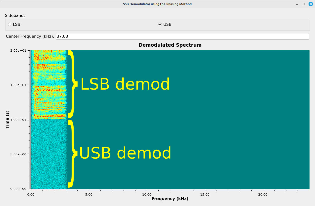
To summarize the phasing method demodulator, it will not only work on a SSB transmission, but it will work on a SSB transmission that is right up against another SSB transmission. You can have multiple USB transmissions all packed into a bit of spectrum, and the phasing method would be able to recover each individually.

Further, the phasing method demodulator will also work on independent sideband (ISB) transmissions. If you tune this to the center of the ISB transmission, it will extract the LSB and USB independently and without one interfering with the other.

Weaver Method Demodulator

The Weaver method demodulator is slightly different from the phasing method demodulator. The difference is that the block diagram of the Weaver demodulator doesn't change from the modulator. Instead, two values change. Those are the values for the frequencies of the local oscillators used to drive the two complex sinusoids. Specifically, the changes required are:

Swap the frequencies of the local oscillators between the two oscillators. The first oscillator becomes the one to downconvert to baseband, and the second one becomes the one to shift half of the bandwidth.
The first oscillator's frequency is inverted (made negative) since it is shifting down in frequency.

Everything else stays the same. Mind you, this is different than several of the papers on the Weaver method I read. For starters, one paper suggested that the first complex sinusoid be a positive sine wave, not a negative⁵. This means that, from the real-signal perspective, we're going to use the negative frequency signal as opposed to the positive frequency one. Given that pretty much every SDR I have will downshift the positive frequency version, I decided to setup my signalling to assume that. That way, when I do finally plug in a SDR, I won't have to change the signs at any point. It should just work.

Block diagram flowing from left to right. The input is marked SSB and splits into two, horizontal branches, one along the top and one along the bottom. The input passes through a multiply, a filter and then another multiply. In the middle are two sinusoidal sources connected to the multipliers. On the right, the diagram is marked Audio. — Block diagram for the Weaver method demodulator. The general flow consists of mixing with a complex sinusoid which brings the signal down to baseband so that the desired sideband (LSB or USB) is centered at 0 Hz (not off-centered as would happen with the phasing method), filtering of the sideband, then shifting of the signal back so that it is off-centered. Because this is not a complex multiply (even though it is a multiply by with a complex sinusoid), the output complex signal will not be usable in any form. Rather, the two branches (I and Q) have to be added (LSB) or subtracted (USB) to get the final signal.

Block diagram of a Gnu Radio flowgraph flowing from left to right. The left-most block is marked File Source, passes through a Throttle block, then splits between an upper horizontal branch and a lower horizontal branch. Each branch passes through a multiply block, a lowpass filter block, and then another multiply block. The multiply blocks are connected to two signal sources. The last blocks on the right are a spectral display and audio output. — Gnu Radio flowgraph implementing the Weaver method demodulator. The signal is split into I and Q branches. The first section multiplies the input SSB signal with a complex sinusoid. The frequency of the sinusoid is such that the desired signal (LSB or USB) is shifted to be centered at 0 Hz. The follow-on lowpass filters pass only the desired sideband. The last set of multiply blocks shift the signal back off-center. The multiply is with a complex sinusoid, but it is not a complex multiply. Therefore, the output of the last multiply blocks cannot be used individually. The output needs to be summed (the Add block) to extract the audio.

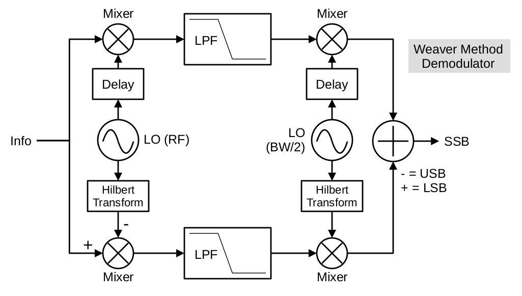
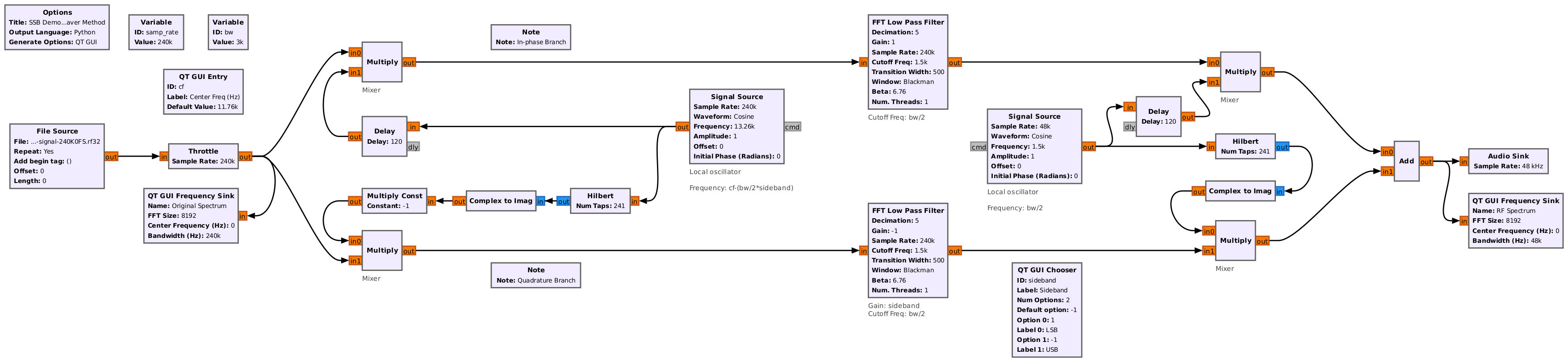
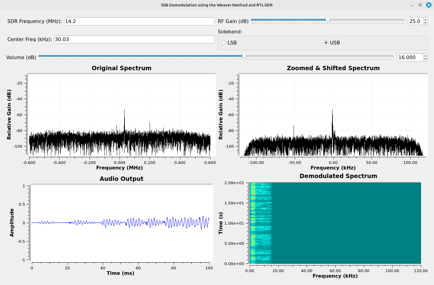
Going through each of the sections of this demodulator, just as we did with the phasing demodulator, we can see how the spectrum changes.

Block diagram of a Gnu Radio flowgraph flowing from left to right. The left-most block is marked File Source (with an output marked 1), passes through a Throttle block, then splits between an upper horizontal branch and a lower horizontal branch. Each branch passes through a multiply block (output marked 2), a lowpass filter block (output marked 3), and then another multiply block (output marked 4). The multiply blocks are connected to two signal sources. The outputs of the second multiply blocks are connected to an Add block (output marked 5). The output of the Add block is connected to a spectral display and audio output. — Gnu Radio flowgraph of the Weaver method demodulator. Each section is marked with a number for the following spectral displays.

Complex spectral display showing two signals shifted towards the left. The signal on the right is centered at 0. — Point #2) Complex spectrum of the complex shifted spectrum. The positive frequency LSB signal has been shifted to 0 Hz. Note that, unlike the phasing demodulator, the Weaver demodulator doesn't shift the signal so that it is off-center from 0 Hz. Rather, the signal is shifted so that the sideband is centered at 0 Hz. The shift has to take into account the sideband being demodulated.

Spectral display showing a LSB signal centered in the spectrum, and filtered so that it is the only signal present. — Point #3) Spectral display of the output of the lowpass filter. Unlike the phasing method, the lowpass filter of the Weaver demodulator only passes one sideband (the phasing demodulator passes both).

Spectral display showing a double-sided signal. — Point #4) Spectral display at the output of the multiply. This double-sided spectrum shows the SSB signal after it has been multiplied by the complex sinusoid. If you convert this to a real, audio signal, it will (probably) be legible audio, but it will always sound as if it is off-tuned.

Spectrogram showing a mostly empty spectrum except for a column on the left. The top half is relatively flat. The bottom half shows a varying audio signal. — Point 5) Spectrogram showing the final, demodulated signal with settings for both USB (top half) and LSB (bottom half). Note that when the setting is different from the sideband (USB selected for a LSB signal), nothing shows up. This is due to the fact that, when the opposite sideband is selected (and assuming no signal is present where the other sideband should be), the other sideband will be filtered out.

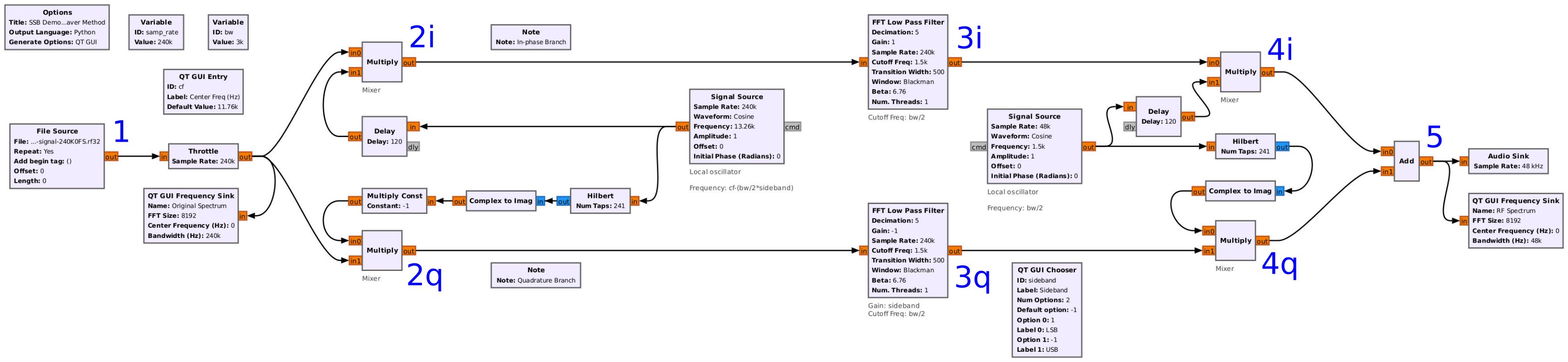
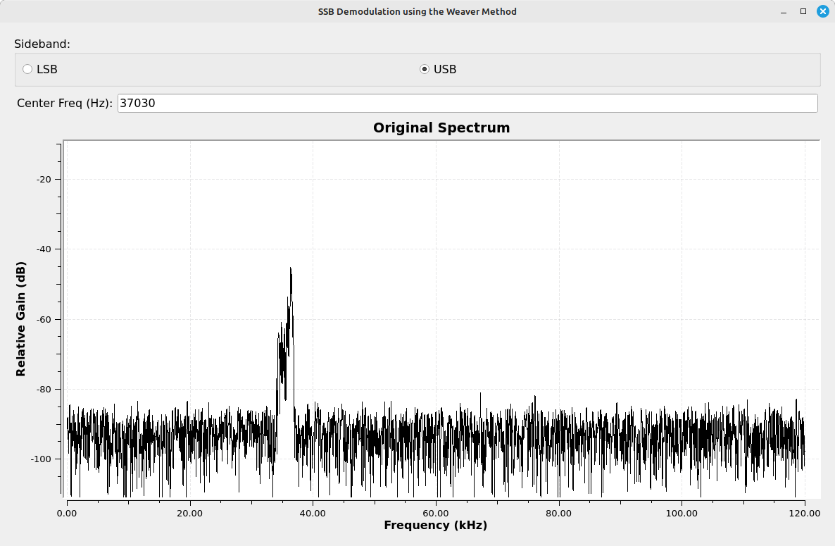
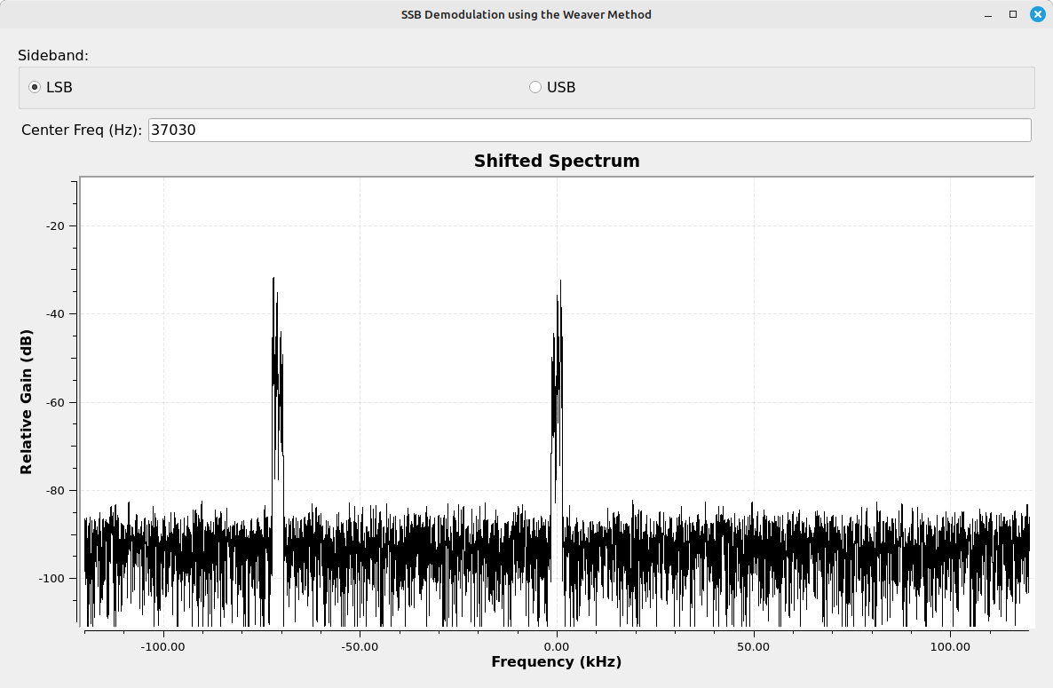
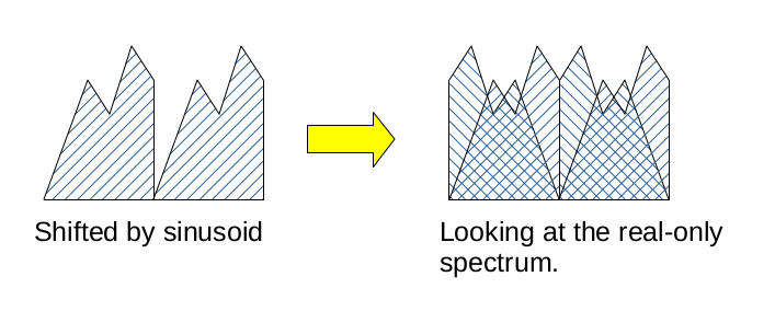
Look at the spectrum of point #4. After the second multiply with a complex sinusoid, and just before the Add block, each branch shows a double-sideband signal. Here's the interesting part. Each of those sidebands is actually the original, desired sideband, but overlapped with the spectrally-inverted version of itself. That's due to the fact that the original, SSB signal is centered at 0, then is mixed with a cosine (I branch) and sine (Q branch). When treated as real, this will shift the signal higher in frequency so that it is just offcenter, but it will also shift it down slightly. And due to the fact that this is still a real signal, each of these sidebands requires symmetry. Hence, the final signal is both the original sideband plus a spectrally-inverted version of itself.

On the left, two single sideband, lower sideband signals right next to each other. The words shifted by sinusoid sit beneath them. An arrow points to the right. On the right, each sideband is overlapped with a spectrally-inverted (flipped left-to-right) version of itself. — Spectrum of the single sideband signal when it is overlapped with a spectrally-inverted version of itself.

	This is the demodulated audio from the I branch of the Weaver demodulator (point #4i in the diagram above). Note that it is legible audio, but regardless of adjusting the center frequency, it will not sound correct. This is due to the fact that the audio is overlapped with a spectrally-inverted version of itself.
	This is the demodulated audio from the Q branch of the Weaver demodulator (point #4q in the diagram above). It is similar to the I branch.
	This is the demodulated audio from the Weaver demodulator (point #5 in the diagram above). This is after both I and Q branches have been added. Because of the phasing, the spectrally-inverted versions will be removed.

I modified the flowgraph to incorporate a SDR as the front end (similar to what I did with the phasing method demodulator). I (yet again) used the HackRF One as my SSB transmitter, connected directly (through a series of SMA attenuators) to my SDR (a RTL-SDR).

To wrap up, the Weaver demodulator is similar to the phasing demodulator. It can handle both SSB and ISB signals. It just does it in a slightly different way.

Demodulator Summary

Let's recap the three, discussed methods for analog SSB demodulation.

Filtering Method: This is a straightforward filtering of the desired sideband and downconversion. Done.
Phasing Method: This uses a combination of complex mixing and the Hilbert transform to recover the desired sideband.
Weaver Method: This uses a complex mixing, a lowpass filter, and a multiply with a complex sinusoid.

As stated previously, the filtering method is the most straightforward. The disadvantage, from an analog perspective, is that it requires a relatively high Q filter (meaning one with a narrow transition width).

Both the phasing and Weaver methods start with the same sections, a complex mixing and a lowpass filter. The difference is two-fold. First, the phasing method tunes so that the SSB signal is off-center from 0 Hz. In other words, if it is a LSB signal, the sideband will extend from 0 Hz down to whatever negative frequency it fits for its bandwidth. The Weaver method tunes so that the desired sideband is centered at 0 Hz, with half of the bandwidth extending into the positive spectrum and the other half extending into the negative spectrum. Second, the phasing method passes both sidebands simultaneously through the lowpass filter. The Weaver method passes only the desired sideband through the filter.

Because of the differences at the output of the lowpass filters for the phasing and Weaver methods (phasing off-centered, Weaver centered), the output is processed differently. The phasing method is Hilbert transformed, and the Weaver method is multiplied by a complex sinusoid. The output of these last sections (Hilbert transform for phasing, complex sinusoid multiply for Weaver) creates a double-sideband signal. The difference here is that, for the phasing method and assuming an ISB signal, both sidebands are still present. As a matter of fact, the audio at the output of either the last delay (along the I branch at the top) or the Complex to Imag block (along the Q branch on the bottom) would have both sidebands present and audible. It would just sound like an audio track with both audio signals present. For the same ISB signal with the Weaver method, there would only be the audio from one sideband (since the other would have been filtered out), but the audio at this same point would sound... not so good.

The signals from the I and Q branch have to be either added or subtracted to recover the original audio (without the other present, or without sounding like an off-tuned SSB receiver). For the phasing method, the addition or subtraction will reinforce the desired sideband, and remove the undesired one. For the Weaver method, the addition or subtraction will cancel the spectrally-inverted signals so that the final audio output is correct.

Which is where we review the advantages and disadvantages of each. There are three circuits that drive the differences. These are:

Filter: As we discussed, analog filters are driven by their Q factor. The issue with the filtering method, either for transmission or reception, is the requirement for a high Q factor filter.
Equal mixers: Both the phasing and Weaver methods require multiple mixers. Both the phasing and Weaver method demodulators start with a complex mixer, which requires two mixers working together. Both have to have equal gain in order not to create IQ imbalance. The Weaver method uses another mixer pair at the end. Again, these mixers have to have equal gains.
Hilbert transform: The Hilbert transform requires that an input signal be precisely shifted by -90 degrees. No more. No less. Even a variation of a degree will limit the attenuation of the mirror image (meaning limit the stopband attenuation of the negative frequency filter).

In short, the phasing and Weaver methods utilize complex signal processing. Such processing is possible (analog television utilized complex signal processing for color transmission and reception starting in the early 1950s), but it is not as easy as with digital signal processing. It's quite possibly for this reason that Miller stated⁶ that filtering was much more popular than either phasing or Weaver.

The Basic SSB Demodulation

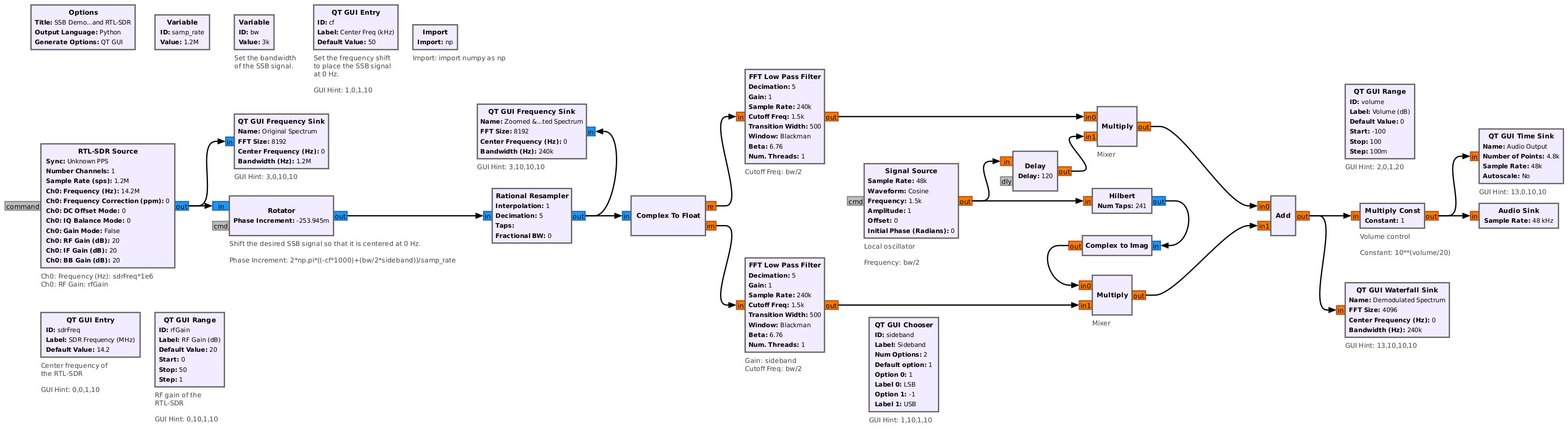
We've gone through several analog methods for demodulating SSB signals. Now, let's look at a method for receiving SSB signals that utilizes DSP techniques. We'll build a Gnu Radio flowgraph to do just that. We're going to use the filtering method, similar to the filtering demodulation method discussed above. The difference is that we're going to use complex signal processing, not real-only signal processing.

Block diagram of a signal flowing from left to right. The input block is marked RTL-SDR Source, which passes into a block marked as frequency shifter. The RTL-SDR Source also connects to a spectral display and time sink. The output of the frequency shifter connects to a resampler, followed by a filter, complex-to-real and an audio output. Various blocks around the perimeter have controls for frequency, gain, and sideband selection. — Gnu Radio flowgraph to implement a SSB receiver using complex filtering. The source is a RTL-SDR, but could be pretty much any SDR. The output of the RTL-SDR passes into a Rotator block, which is used as a frequency shifter. The output of the shifter passes into a Rational Resampler, which drops the sample rate for further processing. The output passes through a complex filter which passes only the desired sideband. The filter output passes through the Complex to Real block, which converts the signal to real for the Audio Sink.

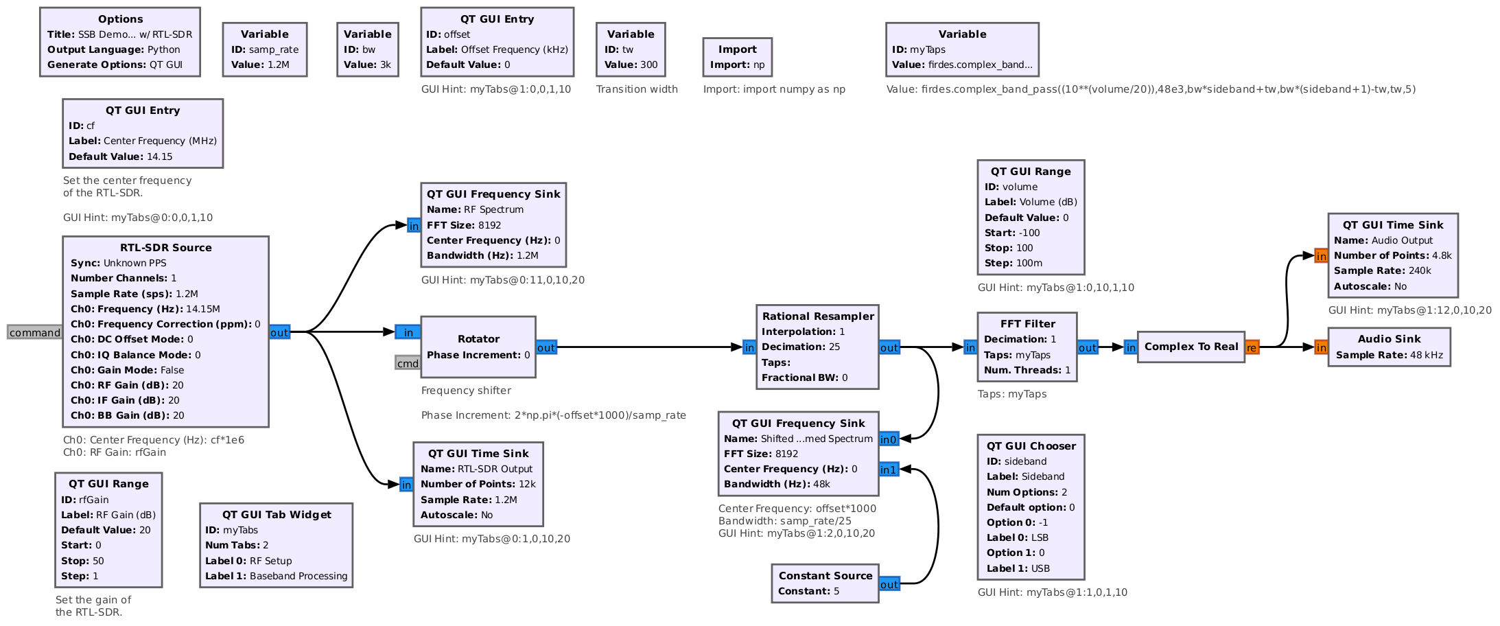
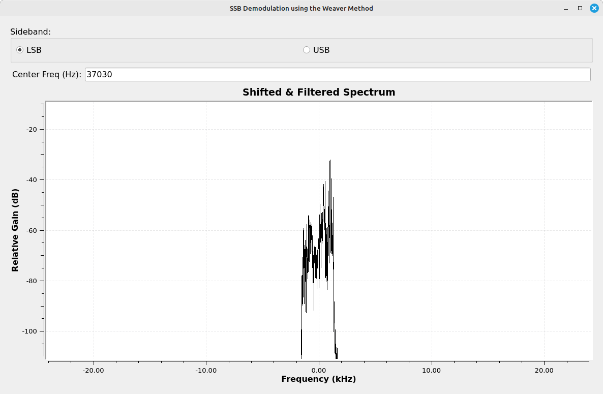
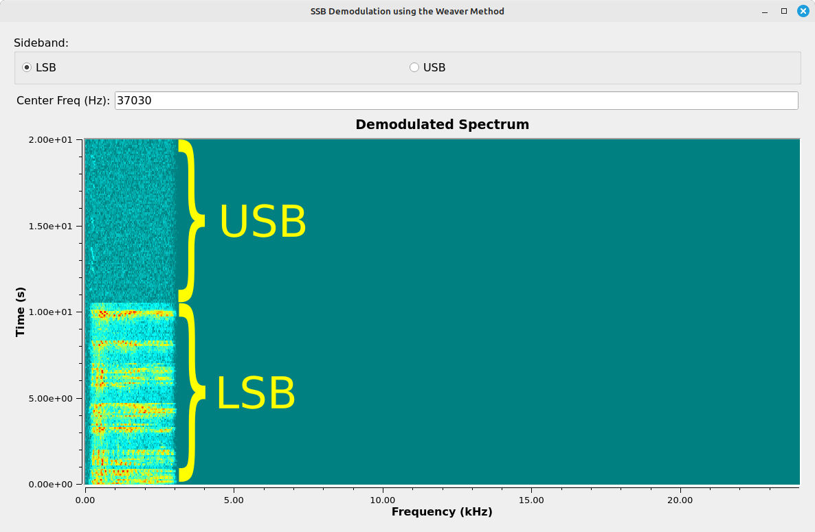
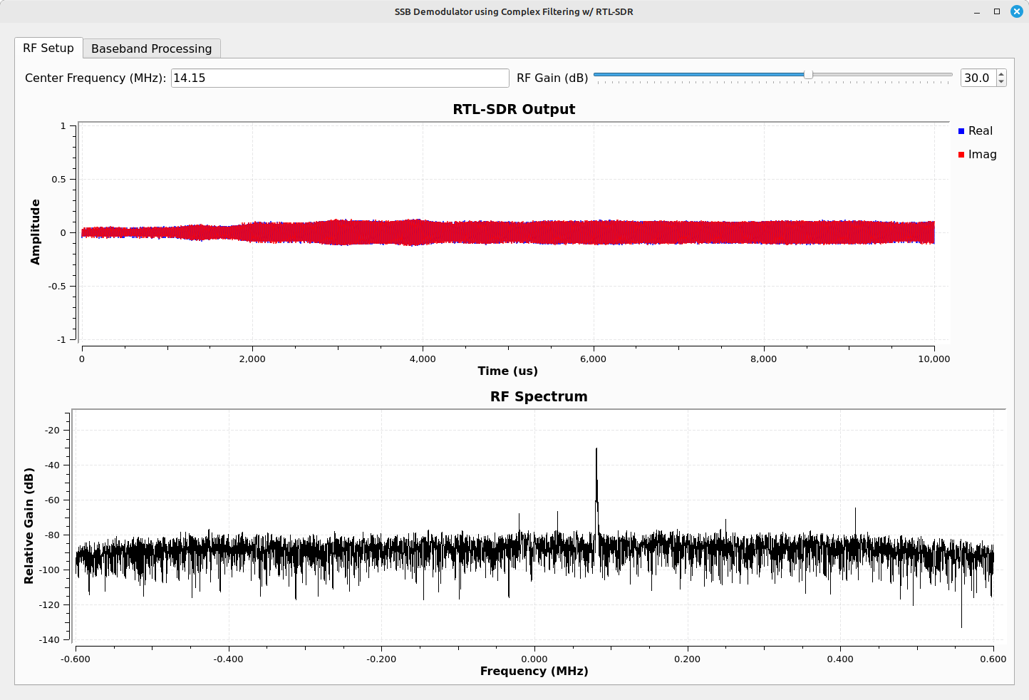
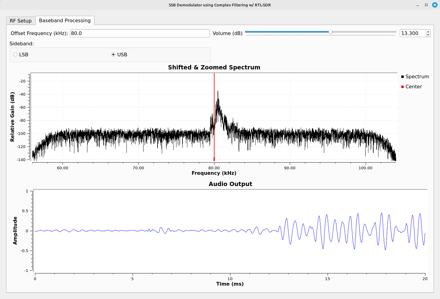
I once again setup a HackRF One as my SSB transmitter. (NOTE: Again, the connection is direct connected between the HackRF One and the RTL-SDR.) Running the flowgraph gives me the following screens:

Display showing a time domain display on the top and a frequency domain display along the bottom. Controls for the frequency and gain run horizontally along the top. — Display that opens up when the flowgraph is first run. The top display is a time domain display of the samples coming directly off of the RTL-SDR. It can be used to adjust the gain of the RTL-SDR for the best sensitivity. The bottom display shows the spectrum being collected by the RTL-SDR, and is used to identify signals to be demodulated. It's used to set the offset frequency on the second tab ("Baseband Processing").

Two horizontal displays, one on top and the other along the bottom. The top display shows a spectrum, marked Shifted and Zoomed Spectrum, of a USB signal. The lower trace shows a time domain signal marked Audio Output. Controls run horizontally along the top. — The second tab, called "Baseband Processing", when the flowgraph is run. This shows the shifted and zoomed spectrum on top, and the amplitude going into the audio sink along the bottom. The controls along the top allow the user to set the offset frequency (determined from the first tab), the type of demodulation (LSB or USB), and the audio volume.

This flowgraph is not optimal. Gnu Radio is designed for prototyping, not for designing a system with the perfect user interface. However, the underlying logic (frequency shifting, filtering) should be sound. It also works. Given that the bandwidth is only that of the SSB signal, it should be optimal for sensitivity.

And there you have it. I hope you found this useful, because I. Am. Spent!

References

1 "Amateur Radio and the Rise of SSB", Gil McElroy, ARRL QST Magazine, January 2003.

2 "Modern Electronic Communication (Seventh Edition)", Gary Miller & Jeffrey Beasley, Prentice-Hall, 2002.

3 "Principles of Communications: Systems, Modulation and Noise (Second Edition)", R.E. Ziemer and W.H. Tranter, Houghton Mifflin Company, Boston, 1985.

4 "Understanding the 'Phasing Method' of Single Sideband Demodulation", Rick Lyons, DSPrelated.com, 8 Aug 2012.

5 "Weaver SSB Modulation/Demodulation - A Tutorial", Derek Rowell, February 18, 2017.

6 "Handbook of Electronic Communication", Gary M. Miller, Prentice-Hall, Inc, Englewood Cliffs, NJ, 1979.

Random Quote Board